The project aims to build familiarity and intutiution for working with convolutions and its applications such as derivatives and frequency filters. We will apply these techniques to make many different interesting outcomes based around techniques such as hybrid images and image blending.
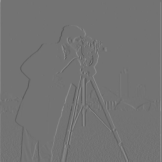
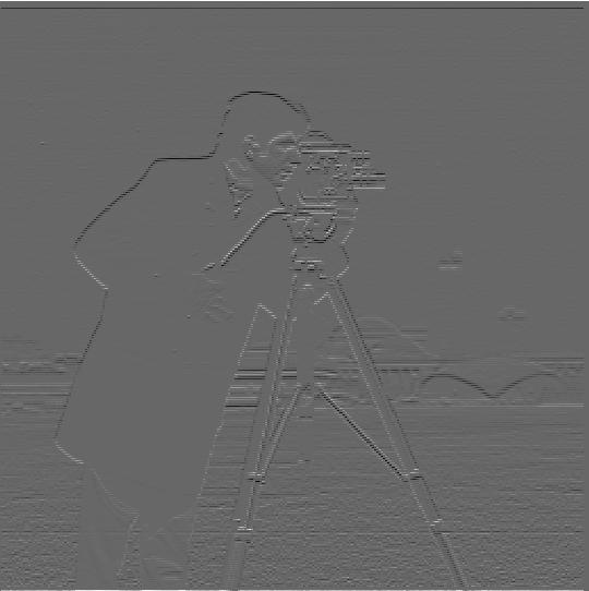
Here we are applying the finite difference operator to simulate taking (partial) derivatives of an image. When convolved with an image, the finite difference operator works by finding the difference in neighbouring pixel values in the relevant direction (ie either x or y direction depending on whether the D_x or D_y filter is being used), which is an approximation to the derivative. Approximating--rather than precisely calculating--the derivative is necessary when working with digitized images, since digitzed images (when viewed as a function Z^2 -> R) are only defined on integer values ( as Z^2 is the domain) while the typical notion of taking derivatives requires the function to be defined a more continuous domain such as R or C. Thus, we can not perform the typical limiting process as we can not compare function values arbitrarily close to each other to approximate the slope. Since the closest values we can compare are neighbouring pixels, the finite difference operator will be one of the best approximations we can get to the derivative.
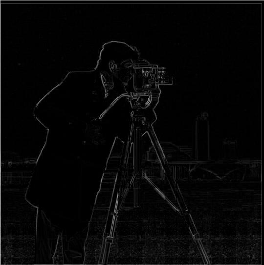
Let's look at the partial derivatives of the famous cameraman image using the finite difference operator. On the right is the derivative magnitude image, which shows the mathematical magnitude of both partials together at each pixel. To be precise, the derivative magnitude is the L2-norm squared of the gradient vector [dx, dy] at each pixel, where dx is the partial derivative with respect to x and dy is the partial derivative with respect to y.


Derivatives can be useful in finding edges, a technique I used in project 1. In images, edges are correlated with gradient magnitude, so pixels with larger gradient magnitude are more likely to contain an edge in the image. To determine what is an edge, the images below are the result of defining a certain cutoff that a gradient magnitude must exceed in order to be an "edge". Finding the appropriate cutoff is rather subjective and can be found via trial and error. I tried many different cutoffs to see which one best captured the edges in this image. Below are a few of the interesting cutoffs.
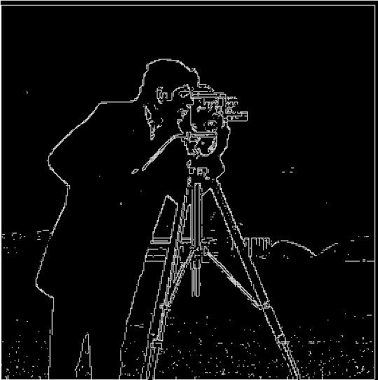
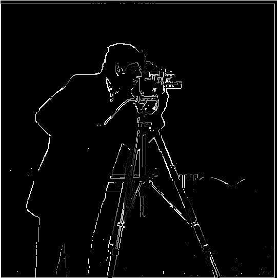
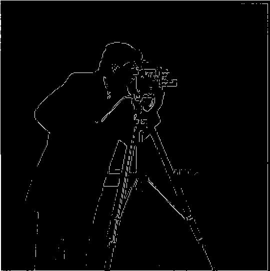
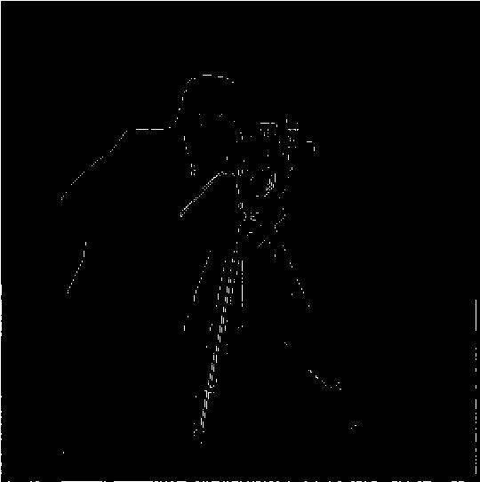
Finding the appropriate gradient magnitude cutoff is a balancing act of trying to minimize the amount of noise that is picked up as an "edge" while still classifying true edges as "edges". Higher cutoff values will allow less noise to be classified as an edge; however, too high of a cutoff value will eliminate too many true edges. In my opinion, the cutoff of 35 allows too much noise to pass through as an edge, while the cutoff of 100 eliminates too many true edges despite doing a good job of reducing noise. Thus, I think that the cutoff values of 50 and 70 are reasonable and do a good job of balancing both of our objectives. I would choose the cutoff value of 50 as my favorite, since it retains edge information on the camera itself, some of which is lost in the cutoff of 70 image.
As I noted above, the derivative images above are quite susceptible to noise. This is because noise presents itself as a fast change in a few pixels, which will be picked up by our small original D_x and D_y filters. Thus, we turn to our old friend: the Gaussian filter. The Gaussian filter removes the high frequency components of our images. Since noise is a fast change over a small spatial area, it is a high frequency signal. Thus, the Gaussian filter will remove noise from our photos. This also makes sense when you consider what a Gaussian filter is doing spatially: it is taking a weighted average of the surrounding pixels. Thus, any noise that is in just a small number of pixels will be insignificant and will not contribute much to the average that determines the smoothed pixel value.
That being said, let's try applying the Gaussian filter to our image before the derivate it in order to remove noise from our edge detectors. Here I am using a 20x20 Gaussian kernel with a sigma value of 3.3. I chose this sigma value to be such that 6*sigma roughly equals 20. Since almost all of the measure of a Gaussian kernel lies within -3 standard deviations to 3 standard deviations, this ensures that the vast majority of the Gaussians measure is being captured in the kernel and that there are few values in the kernel that are essentially 0. These traits help us with the objectives of smooth filtering and computational efficiency respectively.
To create the kernel, I got a 1D 20 length Gaussian kernel from openCV2's getGaussianKernel() function and performed an outer product on it with itself to generate the Gaussian kernel.
Below are the results of taking the derivatives of the Gaussian filtered cameraman:
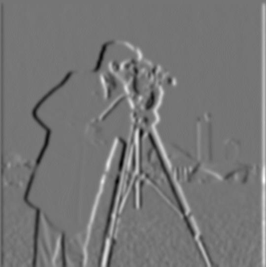
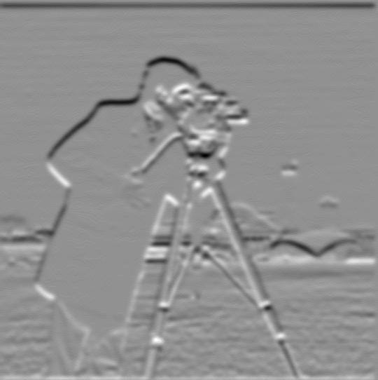

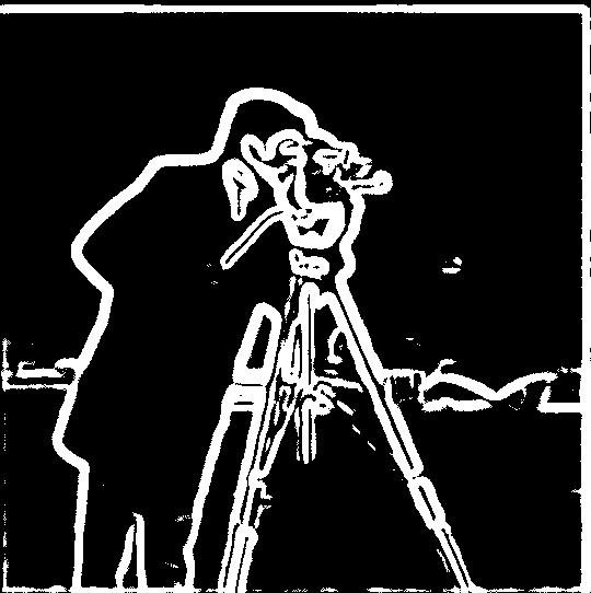
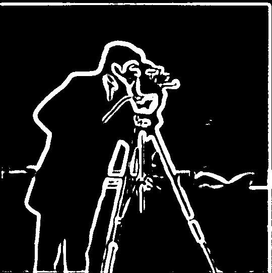
Unsurprisingly, the derivatives of the blurred camerman look blurred. This results in thicker edges, deeper appearing edges, and reduced noise. In partituclar, I can see that some of the lesser edges in the lower right quadrant are much more noticable in the derivative of the blurred cameraman. I hypothesize that this is due to the edges being very thin in the unblurred image. Despite being thin, these edges are not filtered out in the blurred image since they are relatively long. The blurring makes these edges wider, and thus wider in the derivative. Overall, these factors lead to the derivative of the blurred image being much more asthetically pleasing than the derivative of the raw image.
Notice that our implentation of blurring and derivation are both using convolution. In particular, we are doing image --convolve with Gaussian filter--> blurred image --convolve with finite difference filter--> derivative of blurred image.
One lovely property of convolution is that it is associative. As a result, we can reduce our workflow's complexity from doing two convolutions to doing a single convolution with a filter that is the Gaussian filter convolved with the finite difference filter (known as Derivative of Gaussian filter or DoG). Let's put this to the test! Below are the results of convolving the cameraman image with the DoG filter. They should be identical to the derivatives of blurred cameraman images above.


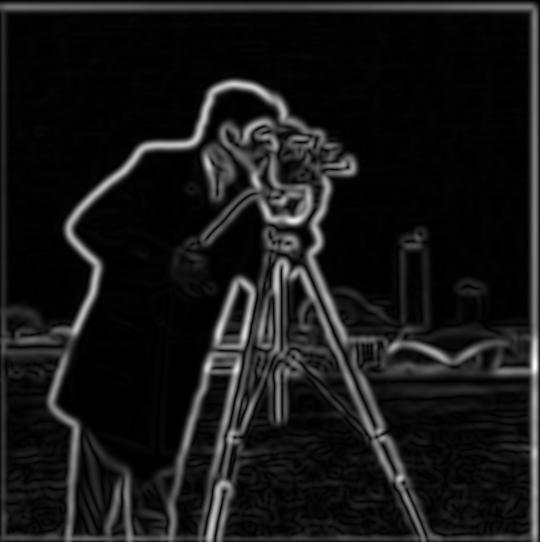
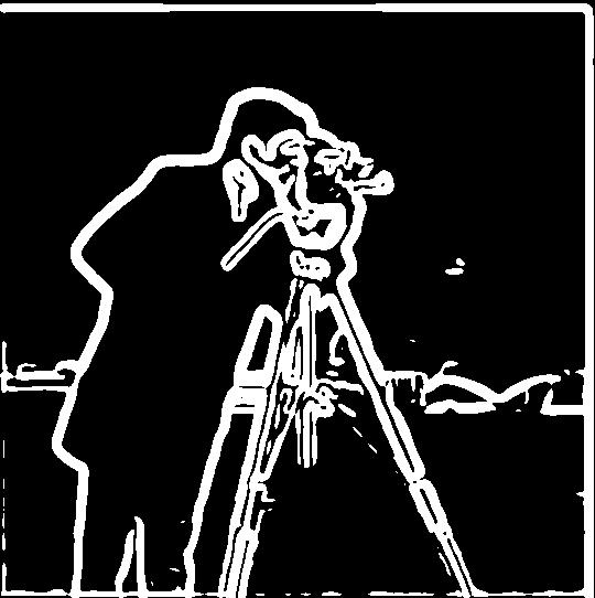
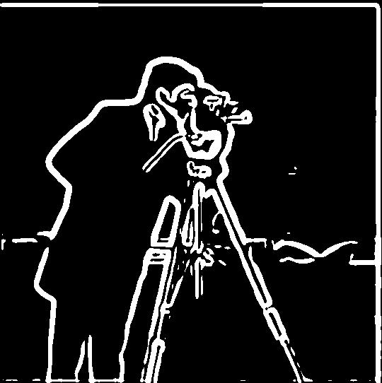
To me, the DoG cameraman images look extremely similar to the derivative of blurred cameraman images above.
In this section, we are sharpening images using unsharp mask filtering. As described in the project intro, low-pass filtering (such as by convolving with a Gaussian filter) removes the high frequencies from images. Thus, subtracting the low-pass filtered image from the original image will yield the high frequency component of the image. To sharpen the image, we want to add more high frequencies back to the image. Thus, we should add the high frequency component found above to the original image to sharpen it. Using properties of convolution, we can acheive this by convolving the original image by the filter (1 + a)*delta - a * Gaussian, where a is a sharpening parameter that controls how sharp to make the image, delta is the kronecker delta function, and Gaussian is an appropriately sized and scaled Gaussian filter. For the same reasons as above, I use a sigma value approximately equal to the size of the Gaussian / 6.
For my sharpening filter, I used a filer of size 21x21 with a sigma of 3.3.
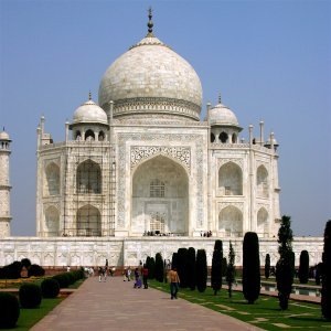
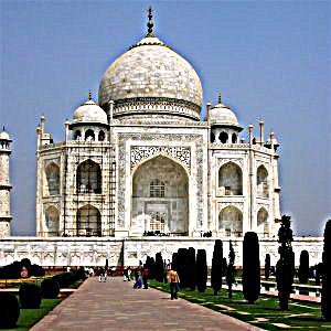
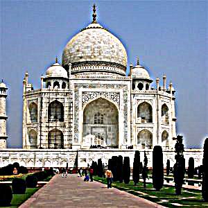
Shown below is the result of applying the sharpening filter to the Taj image with various a values.

Below are the results of applying my sharpening filter to various images that I have sourced. As a test, I will blur various images and apply my sharpening filter to see how much the images can be resharpened. The following images are featured:
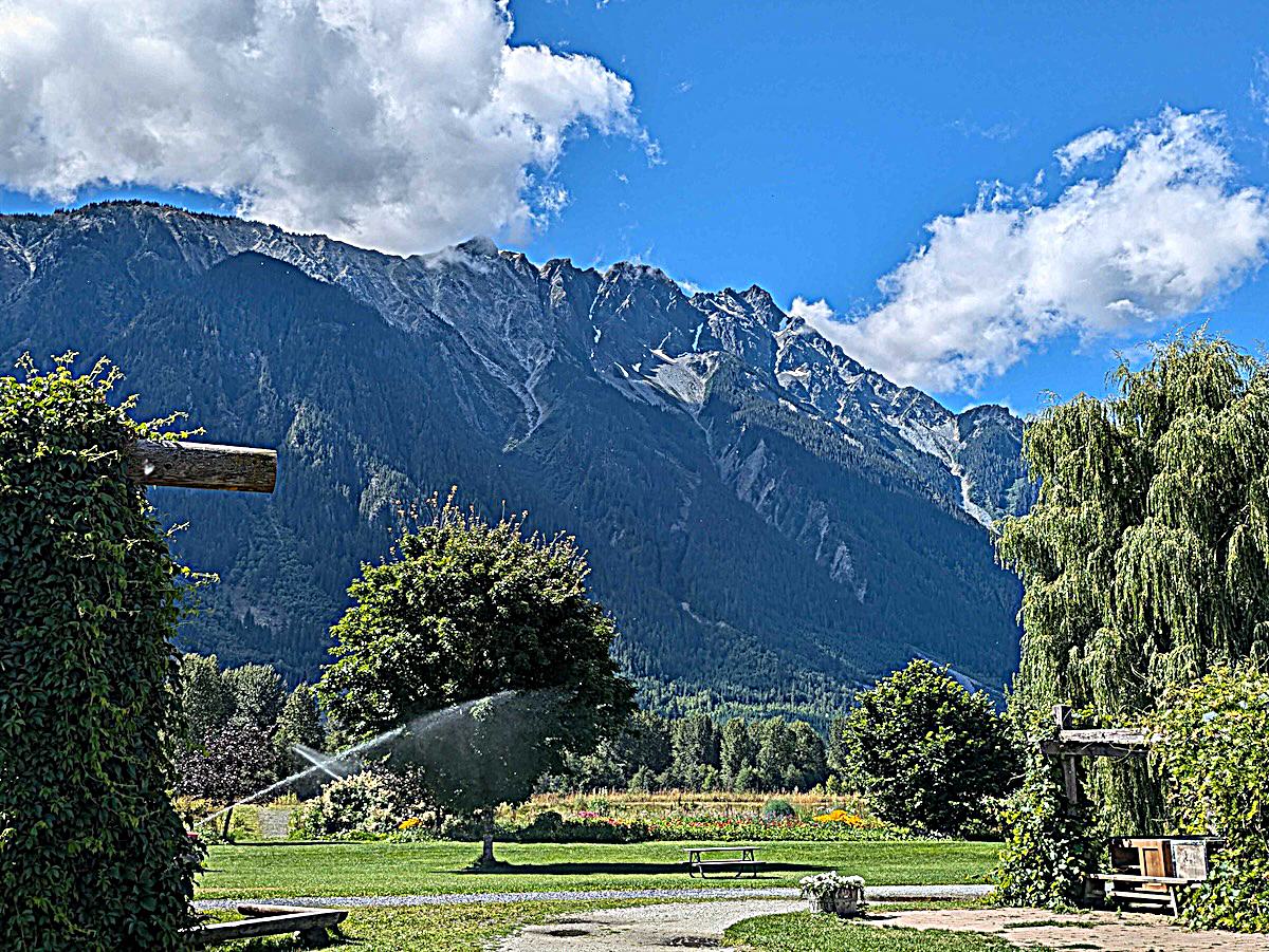
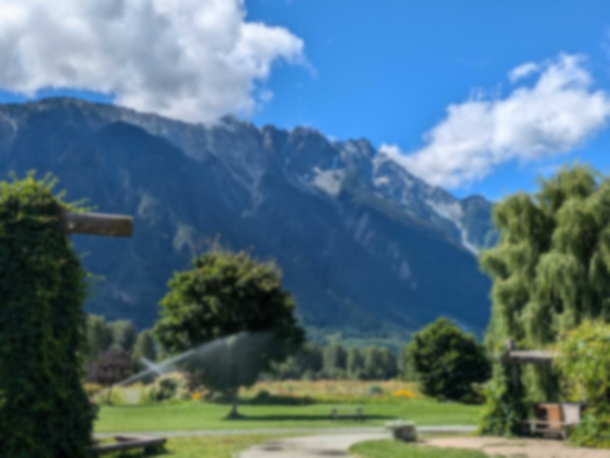
1. An image I took at North Arm Farm in Pemberton, BC this summer. I show both a sharpened version of the original image, a blurred image, and a sharpened version of the blurred image.
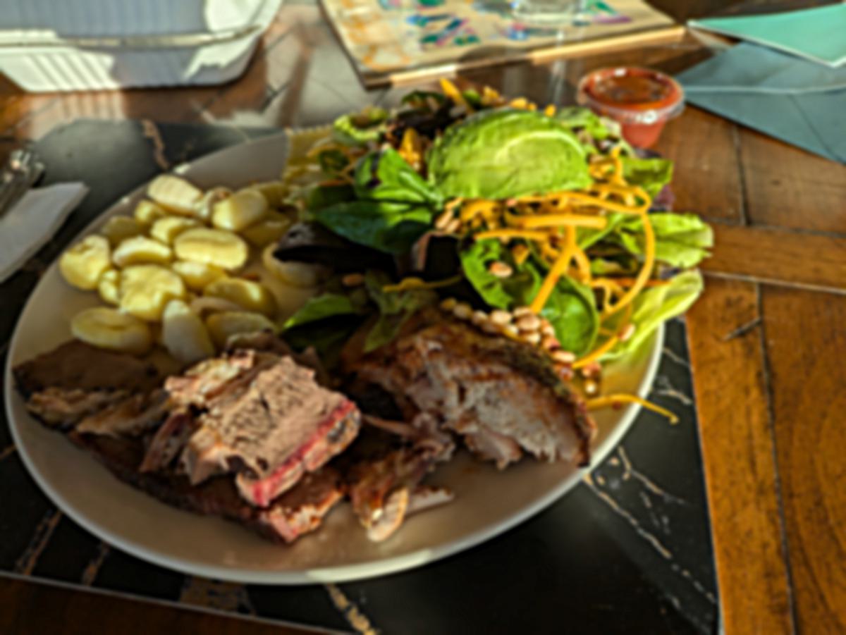
2. A plate of bbq food from my camera roll. I show the original image, a blurred image, and a sharpened version of the blurred image.
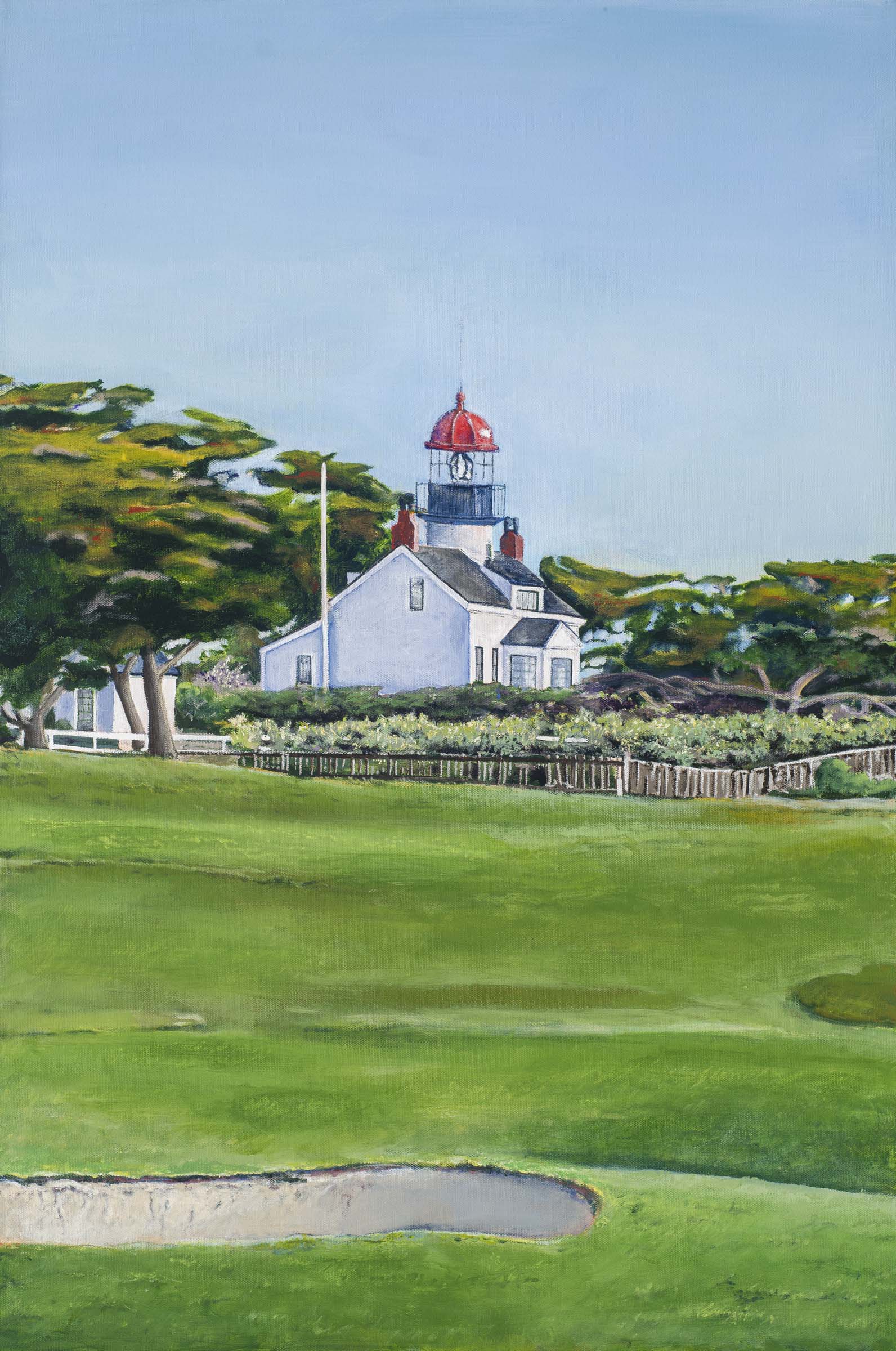
3. A professional capture of one of my mother's paintings. I show the original image, a blurred image, and a sharpened version of the blurred image.
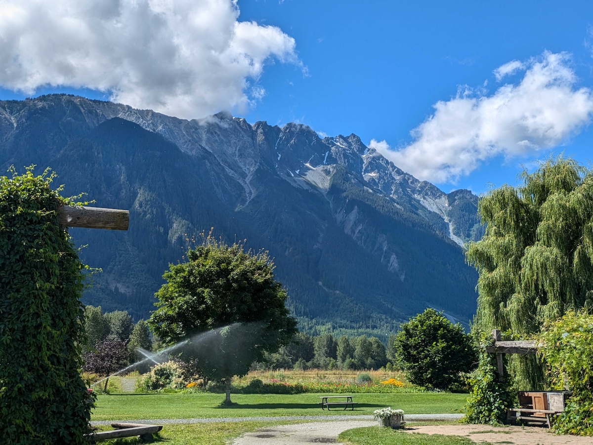



Taj: When the Taj image is sharpened, we can see that high frequency features such as the grid like pattern on the left of the Taj Mahal are much stronger. Likewise, we can see a much clearer definition around the outside edge of the Taj Mahal, creating an almost radiance like effect on stronger sharpening settings.
North Arm Farm: Sharpening the North Arm Farm image strengthens high frequency information around the ridgeline, in the clouds, on the right hand weeping willow tree, and on the water stream from the irragation sprinkler.
When resharpening the blurred image, we can not fully recover the detail of the original image. However, the re-sharpened image is much more realistic and detailed than the original image, especially on the image with sharpening parameter a = 3. Thus, I would call the re-sharpening successful on this image.
BBQ Brisket: Here, the resharpened image does show improvement over the blurred image in being closer to the original image. In particular, the resharpened image regains detail on the grain of the brisket and on the pine nuts in the salad.
Point Pinos Lighthouse: The changes over the variations are lesser in this image than in the other images. We can see that that the sharpened images does a very good job of recapturing detail around the red roof of the lightouse. I expect that this is because the image never contained much high frequency content due to originally being a painting rather than a real world image. Thus, filtering and accenuating high frequencies does not do that much since the image did not originally contain that many high frequencies.
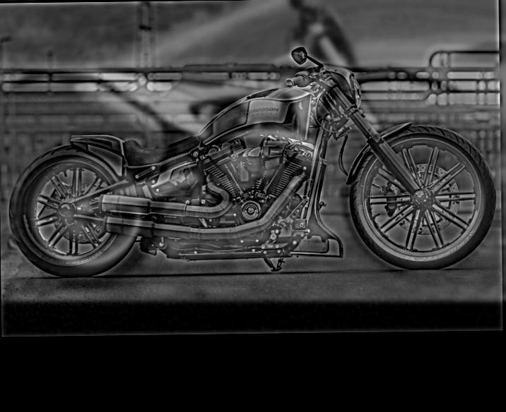
Hybrid images are an oppurtunity to apply what we have learned to generate some cool images. Hybrid images refers to overlay of two different images at different frequencies so that the image appears to be of different objects when viewed at different distances. To start this process, we start with two images would like to overlay, typically converted to grayscale. We first manually align the features of the image, using the align_images code provided by course staff. Next, we apply the 1 - Gaussian filter to one image and low filter another using a Gaussian filter. Thus, we are left with the high frequencies of one image and the low frequencies of another image. When overlaying the two images together, the resulting image has a high frequencies of one image and the low frequencies of another. Since humans primarily percept high frequencies at close distances and low frequencies at far distances, we see one image when viewing close and a different image from looking far away.
Below are some examples of images produced along with the corresponding input images.

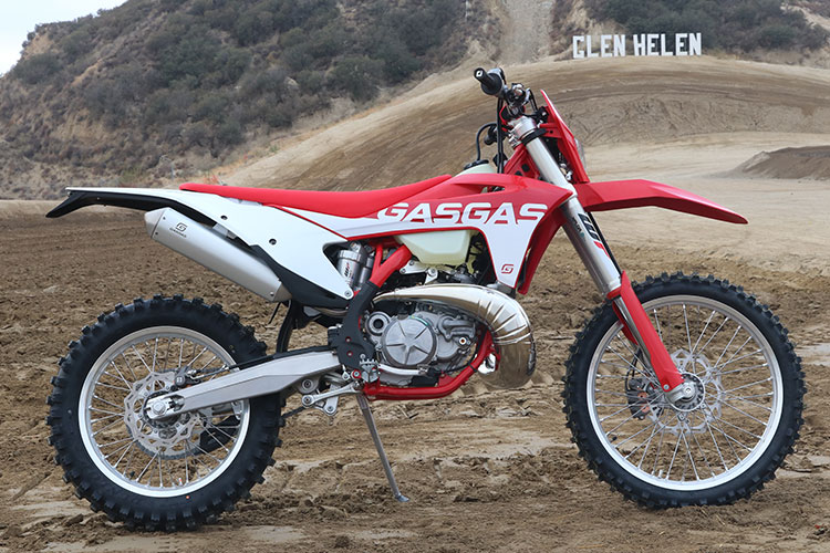
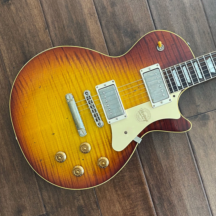
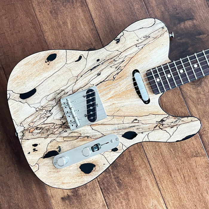
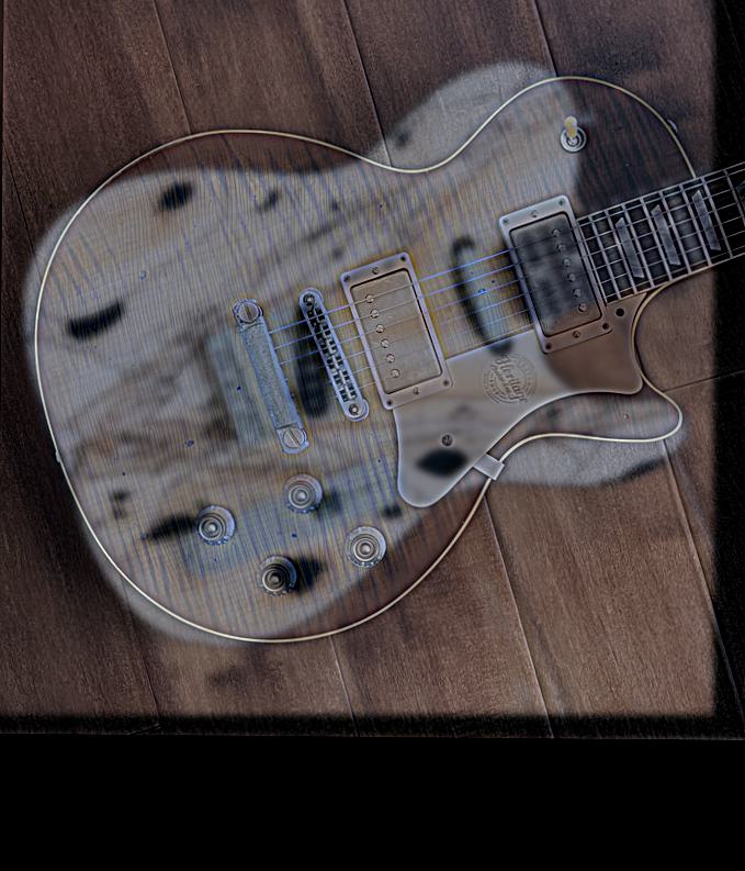
Notice the flame maple pattern shows up very well in the high frequency guitar.

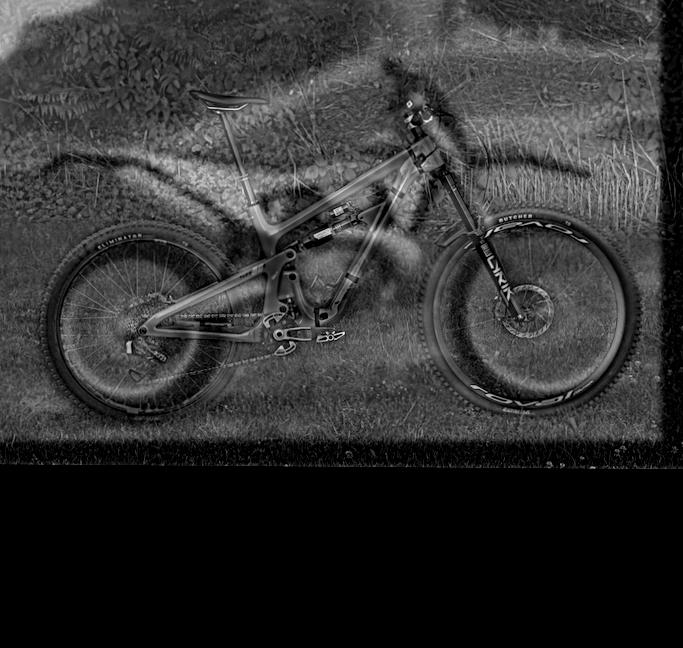
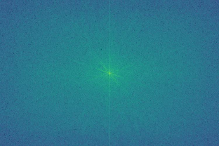
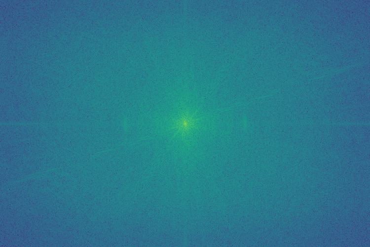
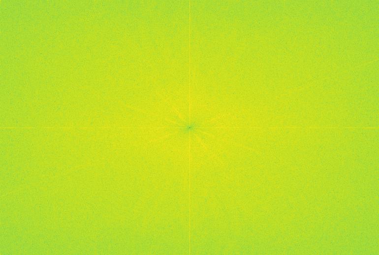

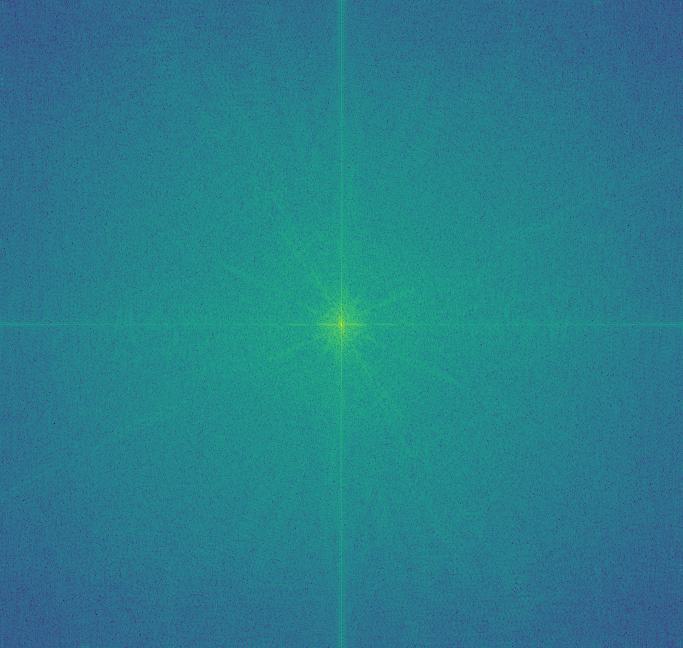

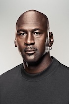
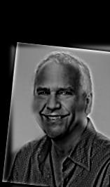
I had a difficult time trying to hybridize these two images. I thought it would be entertaining to do a play on names with the extremely famous UC Berkeley Statistics and CS Prof Michael Jordan and a lesser known Michael Jordan who happens to be a basketball player. I attempt to hybridize the images with the professor in the high frequencies and the athlete in the low frequencies, which is the more successful configuration. Despite this, I was still unable to be completely satisfied with my hybrid image. I adjusted many parameters such as cutoff frequency for both images independently and mixture ratios; however, it seems that, in all cases, one of the two images would dominate the image close and far.
The goal of this section is to create a Gaussian and Laplacian stack. A Gaussian stack is a collection of images (which I store in a 4D tensor for color images) containing the original image on top and progressively more blurred images as we go down the stack. To create each progressively more blurred image, I convolve the previous level's image with a Gaussian filter that grows in size and sigma as we go down the stack. As before, I keep it so that sigma = filter size / 6.
A Laplacian stack is one containing the mid-band frequencies at progressively lower frequencies as we go to lower levels of the stack. Level t in the Laplacian stack is created by taking the difference between the Gaussian filter at level t and the Gaussian stack at level t + 1. This works since the Gaussian stack contains low-passed images, so the difference between the Gaussian filter at level t and the Gaussian stack at level t + 1 contains the frequencies that are high enough to be blurred from Gaussian level t + 1 but not high enough to be blurred from Gaussian level t. Thus, we get a band pass filter. To be precise, the Laplace stack at level 0 contains a high-pass image. Finally, the remaining low-pass image is added to the lowest level of the Laplace stack. This ensures the nice property that the sum of the Laplacian stack is the original image.
As we will see in the next part, we can use these stacks to create blended images. Here is a recreation of the Oraple image from the 80s.
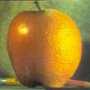
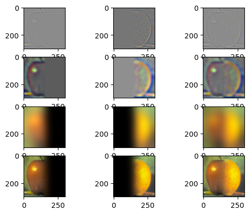
As forshadowed in part 2.3, we can use the stacks to blend two images together without seams. To do this, we need to create a mask. The mask will be a step function that transitions where we want the images to transition. Then we will use the Gaussian and Laplacian stacks that we know how to create from the last section. For the two images to be blended, calculate their Laplacian stacks. Calculate the Gaussian stack for the mask. For each layer in the stack, find the convex combination of that level in the Laplacian stack of each image with the weighting given by the mask of that layer in its Gaussian stack. This combines the high frequency components of the images with a sharper boundary and the lower frequencies of the image with progressively smoother boundaries. Let's look at some results.


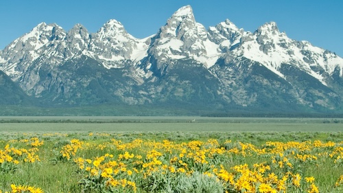
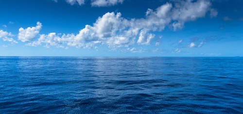
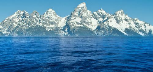
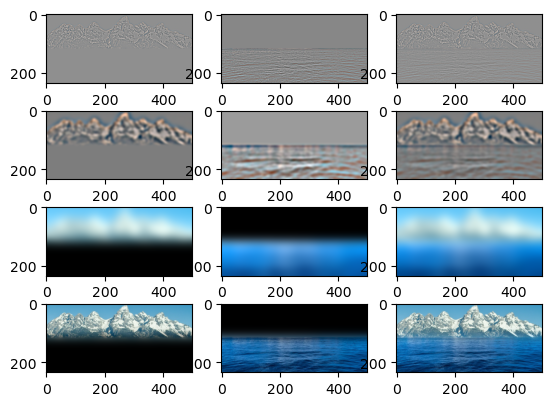

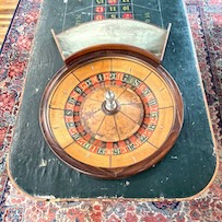
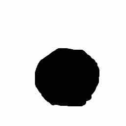
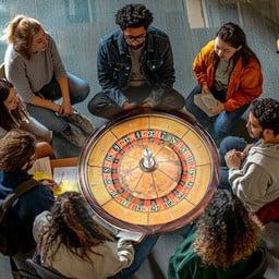
I find the Gambling Students picture I created to be particularly entertaining. I hope it makes you laugh as much as it does me.
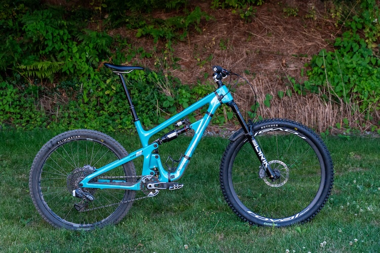
I'll include this following blended image with a custom mask even though it did not turn out too well. For context, the original image is of me mountain biking down an easy rock roll, while the other input image is of a very difficult rock roll. I thought it would be a good use of effort to make a blended photo of myself riding the more difficult rock roll. However, the blended image did not turn out too well, as you'll see. I'll hypothesize why this happened below.
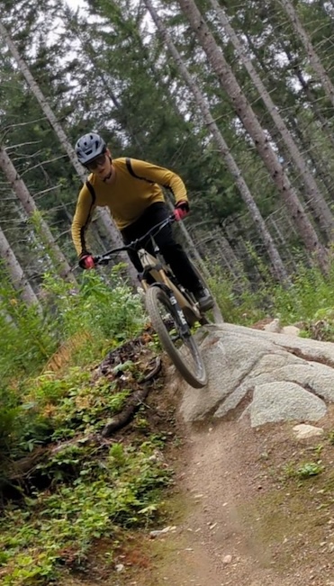
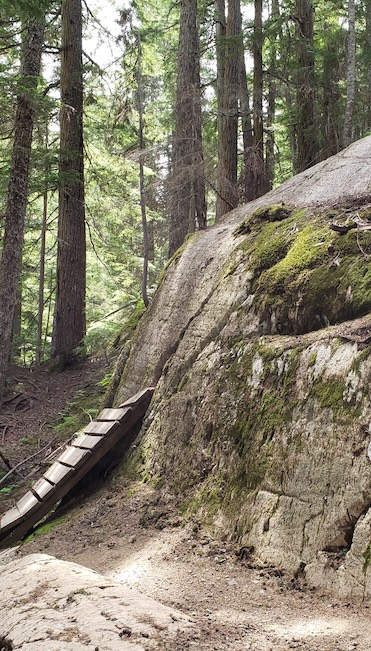
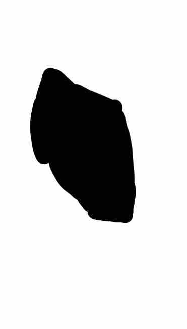
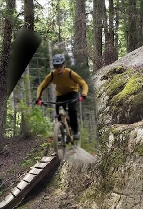
There were several factors that lead to the poor blending. First, I had a difficult time creating the proper mask due to the irregular shape of me and my bike and having to have the images aligned properly first. Second, even with a proper mask, I do not think that the blend would have turned out well, since the forests in the backgrounds of the images are different--the image containing me has smaller and tigher spaced trees than the other image. Additionally, since the rock roll I rode is nowhere near as steep, I am not at the correct angle in the original image of me to match the angle I would be at if I were riding the tough "Manager" rock roll. While I can, and did, rotate the images, the angles the photos were taken at are not compatible. Since the image is 2D, I could not have rotated around the axis needed to align the images. This was not something I initially realized.
The most important thing I learned in the project involved generally getting more experience working with visual image data. In a project such as this that features relatively simple concepts, most of the challenges I faced were debugging issues related to image data structures and data handling and intuition as to which images would be good candidates for blending or hybridization. The additional experience I gained in this project helped me internalize more best practices for working with visual data.
I consulted some external resoures when creating this website for instructions on how to write HTML and CSS code. Some of my webpage code is adapted from https://www.w3schools.com/howto/howto_css_images_side_by_side.asp and https://stackoverflow.com/questions/12912048/how-to-maintain-aspect-ratio-using-html-img-tag.
The description of the blended image progressions in the caption underneath those images is taken from the paper by Szelski.
I would like to emphasize that all of the code for image processing is of my own creation.