
This project works with diffusions models to generate various interesting images with various techniques such as CFG, Anagram generation, and Hybrid images. In part a, we use the DeffFloyd Diffusion model from Stability AI. In part b, we train my own diffusion model to generate MINST digits.
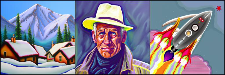
In this section, we are getting familiar with the output of DeepFloyd IF. The model utilizes two stages: the first stage generates 64x64 pixel images and the second stage upsamples the images to 256x256 pixels. For our experimentation, we are using the following three prompts:
[
'an oil painting of a snowy mountain village',
'a man wearing a hat',
"a rocket ship",
].
Each stage has a parameter num_steps that controls the number of iterations the diffusion model uses during the denoising process. Using more steps will generate higher quality images but will be computationally more intensive. I will experiment with the output of each stage for a range of step sizes. Below is the output.


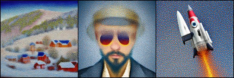

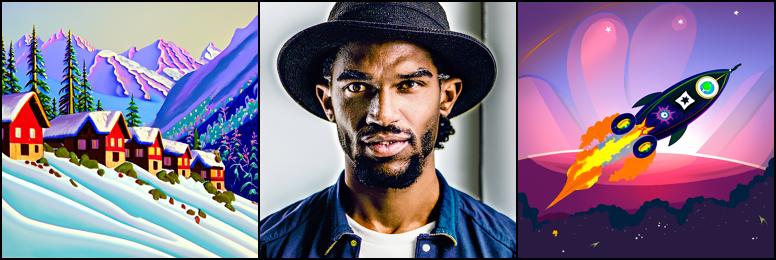
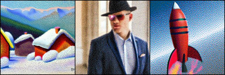

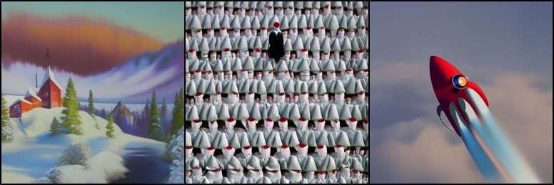

Here we try a variety of combinations of 5, 20, 50 steps in stages 1 and 2. In both stages, I notice a large increase in quality moving from 5 to 20 steps and little quality increase moving from 20 to 50 steps. I also noticed that each stage seems to perform a different task. I infer that stage 1 is responsible for generating the "thoughtful" information content - ie the general content of the image - and stage 2 performs upsampling that increases the image size while keeping the visual content of the image highly similar to the output of stage 1. In particular, we can see that increases in stage 1 number of steps increases the accuracy and detail in the image's visual content while the number of steps in stage 2 controls the pixel quality and sharpness of its output.
For example, inspect the images that result when there are 20 steps in stage 1 and 5 steps in stage 2. These images have stage 1 output that are consistent to the prompt and are feature high qaulity details while the stage 2 output has odd pixels details with poor image quality.
Conversely, consider the images that result with 5 steps in stage 1 and 20 steps in stage 2. The visual content of these images is lacking, supporting the idea that stage 1 creates the visual content. In these images, the mountain village is lacking realism and details in the mountains, the rocket ship is simplistic, and the man in a hat is a rather nonsense image that contains many small hats. However, the stage 2 output with 20 steps is perfectly high quality while retaining the lack of realism in image content from stage 1, which supports the hypothesis that stage 2 determines the upsampled image quality without much effect on visual content.
Throughout this project, I am using the seed 831 with the exception of a few later prompts where I experiment with seed 699 to generate different output. These locations will be noted.
In this section we are noising clean image such that the diffusion model can be trained to denoise them. In this section and following sections, we will be using a photo of the campanile as an clean example image to experiment with. The campanile will be x_0, the clean image at time 0. At time t, the noised image will be solved for according to

Let's see the output of noising. Below are the images we are working with. On the left, is the clean orignial campanile image. To its right, we have the campanile noised at steps 250, 500, and 750.


We know various methods for denoising Gaussian Noise. One such method that we know is Guassian Blurring the noisy images. Lets see how Guassian Blurring handles this noise.

As we can see, Guassian Blurring is unable to denoise the images satisfactorily. In fact, Gaussian Blurring will deliver poor denoising in this situation for any parameter values.
Now, we will try a more sophisticated method to denoise the images. We will use the DeepFloyd Diffusion model from Stability AI that has been trained for these alpha values. DeepFloyd uses text embedding; we will use the prompt "a high quality photo" as instructions to denoise the images. We will be using one step denoising where we call the UNet at the t value used to noise the images to estimate the x_0 clean image. Let's see how the UNet does.
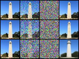
In all cases, the Unet does a generally good job a denoising, certainly better than the Gaussian Blur filter does. We can see that the difference between the denoised output and the original image increases as the level of noise added increases. Since the Unet has to generate more of the image content as the amount of noise increases, this outcome makes sense. Also, the denoised image gets somewhat blurry as the input noise level increases, which is a drawback of one step denoising.
To improve the denoising for highly noised images, we are going to use iterative (multi-step) denoising. DeepFloyd was trained to be used with up to 1000 steps. However, it is not necessary to denoise one step at a time. Instead, we will denoise 30 steps at a time. This allows for us to denoise a noised image noised to at most 990 steps. We can control the starting timestep for denoising with the i_start parameter.
We use iterative denoising to denoise the noisy image of the campanile, which we will compare with our other methods. Below we can see the results of iterative denoising after each 5th loop of denoising, the final clean image after iterative denoising as well as the one step denoised image and the Gaussian filtered image for comparison. Due to ambiguity in the website prompt, I will show the results for denoising from both 690 steps (i_start = 10) and from 990 steps (i_start = 0).


In the last section, we saw how diffusion models can be used to denoise noisy images. However, what will happen if the input image is pure noise? This thought underlies the main use of Diffusion models. Here, we will use this technique to generate new images based on a text prompt. Again, we will use the prompt "a high quality photo" to guide the Diffusion model's image generation. I'll show the results of this strategy in original form and after upsampling and for seeds 831 and 699.


While the above images were decent, some lacked realism or were non-sensical. In this section, we will use a technique called Classifier Free Guidance (CFG) to generate more realistic images. With this techinque, one generates two noise estimates: One will be for the desired (aka conditional) prompt and another for the null prompt "". In this section, we will still use "a high quality photo" as the conditional prompt. The final noise estimate will be calculated as
noise = noise_unconditional + gamma * (noise_conditional - noise_unconditional)
for some paramter gamma. In this section, we will use gamma = 7. During each step, we will iteratively denoise the image according to this noise estimate.
Below are the images generated with CFG upsampled to 256x256 using seeds 831 and 699.


We can see that these images are much more realistic and higher quality than the non-CFG images.
In this section, we will use the CFG techniques we developed to allow the diffusion model to make small edits to images. To accomplish this, we take a clean image, noise it lightly, and have the model denoise it. The result is an image that is similar to the original image, but with some changes as the diffusion model sees fit. We will guide the denoising with the prompt "a high quality image", which provides the model with lots of freedom to edit the image as it sees fit. We will run the algorithm with varying levels of noising, starting at i_start = 1, 3, 5, 7, 10, 20. These values correspond to starting t values of t = 960, 900, 840, 780, 690, 390. I'll apply this algorithm to the test image, as well as two images of my choosing.


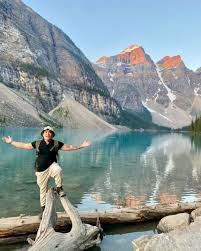
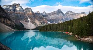
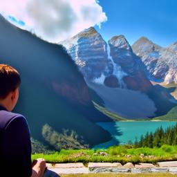
As expected, more noised input images result in translated images less similar to the original image. Utlimately, this algorithm can result in some interesting output images. Additionally, the second-to-right translated image of the North Arm Farm image provides insight into the workings of the diffusion model and its training dataset. Those familiar with the area or Instagram may notice that the translated image is nearly identical to the view of Moraine Lake in Banff, Alberta from a location that is extremely popular with tourists and influencers. I took the original image myself in Pemberton, BC, which is 300 miles from Moraine Lake and is in a different mountain range. Despite these differences, the model decided to denoise the image to one of (essentially) Moraine Lake. This is the first time I have been able to identify a diffusion model output that is actually just a recreation of some real place. I hypothesize that there are so many images of this view of Moraine Lake on the internet--which become part of the Diffusion model training data--due to the horde of influencers that travel there. As a result, the model has a great perpensity to recreate this one exact solution when given an input image remotely similar.
For comparison, I will show a side-by-side comparison of this diffusion model output with a real image of Moraine Lake.
Notice the high number of corresponding features.
We can apply this same technique to images we draw by hand or source from the web. I'll show the output of this method using 2 images drawn by hand and one sourced from the internet.


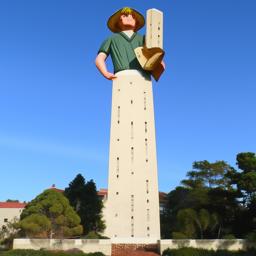
We can extend the methods we used above to only apply edits to certain parts of an image. To accomplish this, we will define a mask where the diffusion model can only edit areas where the mask == 1. Areas that have mask == 0 will not be edited. We will enforce this condition at each step, so the model will have to adjust its changes so that they make sense in context with the rest of the model. We will perform this with the campanile and 2 images of my choosing. Note that upsampling will allow the model to change the entirety of image. I am using seed 831.


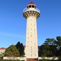


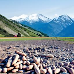


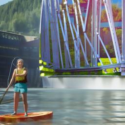
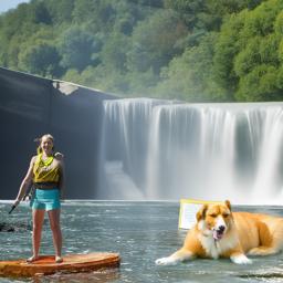
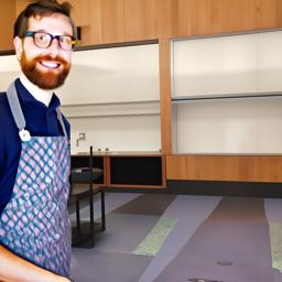
For this section, we will perform a similar routine as in 1.7.3 with the addition of using a different text prompt to guide the changes we desire. I will use a different prompt with each of the test image, and 2 of my own images.
First, we will look at the campanile with the prompt "a man with a hat".


Next, I will edit the web image with the prompt "a photo of a dog".


Finally, I will edit an image of our own lecture hall in Li Ka Shing Center 245. However, at the lectuerer stand is a generation with the prompt "a photo of a hipster barista" in the place than Professor Efros!


Now we will use our expertise in working with Diffusion to generate a visual anagrams. Visual anagrams are an image that will appear as different coherent images when viewed normally and upside-down. To do this, we will need two different prompts--one for the desired outcome at each image orientation. At each iteration, we obtain the noise estimate for the rightside-up prompt on the image and the noise estimate for the upside-down prompt on the flipped upside-down image.
We then perform CFG on both individually, flip the upside-down noise estimate, and average the two to get our noise estimate.
First, let's look at a result of producing an anagram with the rightways-up prompt "an oil painting of people around a campfire" and the upside down prompt "an old painting of an old man".


Next, we will use the rightways-up prompt "a photo of a hipster barista" and the upside down prompt "a photo of a dog". I will include two different generations of the anagram.


Next, we will use the rightways-up prompt "an oil painting of a snowy mountain village" and the upside down prompt "a photo of the amalfi cost". Note that the prompt is "amalfi cost" rather than "amalfi coast" due to a typo in the starter code. Remarkably, the prompt embeddings are robust to these errors, so the images still come out well.


We will now work to create hybrid images using diffusion. A hybrid image is an image that looks different at different viewing distances. In other words, the image will appear to be of different objects when viewed up close and when viewed from far away. We can achieve this by manipulating the frequencies of the image. Viewers will notice primarily the low frequencies from long distances and the high frequencies from short distances. We can thus craft the image's high and low frequencies separately during diffusion iterations to drive the output towards different prompts in the high and low frequencies. To do so, we will have 2 prompts, one for each frequency range. First, we will generate the CFG noise estimates for each prompt. Then we will high pass and low pass filter the respective prompt noise estimates. The sum of the filtered noise estimates will be the noise estimate that we use.
Below is the output following the prompt "a lithograph of a skull" from far away and "a lithograph of waterfalls" from close up. Look at the image from different distances to discern the effect.

Next I'll show two outputs following the prompt "a pencil" from far away and "a rocket ship" from close up.


Next I'll show three outputs following the prompt "a lithograph of a skull" from far away and "a photo of a hipster barista" from close up.


Now we will train our own diffusion model to generate images based on the MNIST dataset.
We will begin by training a UNet to denoise MNIST digits. To do so, we will generate z = x + sigma*eps, where x is the clean MNIST digit, 0 <= sigma <= 1, eps ~ N(0, I), and z is the noised MNIST digit. In this section, we are training the UNet to predict the clean digit itself. During training, x is thus the target and z is the UNet input. The loss is the MSE over image pixels. Further information on the UNet architecture is available here.
To train the network, we are using sigma = 0.5, hidden dimension D = 128, optimized by Adam with step size 0.0001.
Let's see how the model does.
Let's inspect the training process. The plot below shows examples of noised digits for different sigma values. Each row is a different example from the MNIST dataset, and each column corresponds with a sigma = 0, 0.2, 0.4, 0.5, 0.6, 0.8, 1 increasing left to right. The loss plot is also pictured below.
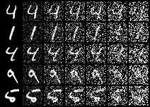
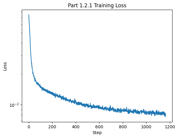
We can see that the loss converged to a small amount consistent with the staff solution.
Below are examples of the UNet's performance after 1 and 5 training epochs. The left column is the original image, the middle column is the noised image with sigma = 0.5, and the right column is the denoised UNet output. Note that the colors are duller due to image processing during the download process rather than from the UNet.


The Unet was trained with sigma = 0.5. What will happen if it is asked to denoise images noised by different sigma values? As it turns out, the Unet performs well with Out of Distribution noised images. Below we noise the same image with each sigma in [0, 0.2, 0.4, 0.5, 0.6, 0.8, 1] and witness the model's output. The top row is the noised image and the bottom row is the Unet output. Each column refers to an increased sigma value (noise level).

Now we have a simple Unet denoiser working, so let's turn to more advanced applications. Here I will implement a diffusion model for MNIST digits with time conditioning and, later, class conditioning. My work in Part B is guided by the DDPM paper. Now, the goal of our model is to transform an input of pure noise into a realistic MNIST output using iterative denoising (aka diffusion). Thus, we will know have the model predict the added noise rather than the output image. We will apply iterative denoising according to the same equation given above:

This model will use T = 300 denoising steps with variance schedule linearly spaced between B_0 = 0.0001 and B_T = 0.02.
First we will add time conditioning to the Unet. This is simple addition implemented by the addition of two FCBlocks as described here.
With our new architecture, we must train the Unet. We are using MSE loss over the pixel values and hidden dimension D = 64. We will train the model over 20 epochs with an Adam optimizer with learning rate 0.001 and an exponential learning rate schedular with parameter gamma = 0.1^0.05. We can see the training loss below, where the model converges well to a loss similar to the staff solution.

We can observe the results of the time-conditioned Unet after 5 and 20 epochs of training.
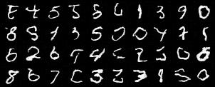
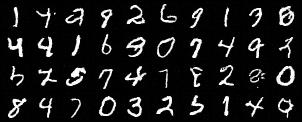
We can see above that the class-unconditioned Unet provides decent results that lack in realism. Much of the issue is that the output appears to be "in-between" different digit values. This makes sense because the Unet does not have direction of what outcome is desired. In this section, we will add class-conditioning to the Unet. When training, we will provide the class of the image, so the network can learn what shapes correspond to certain digits.
When training, we can provide the desired output class to guide the output to a more certain and realistic outcome.
To achieve this result, we will add 2 more FCBlocks to the network that multiply various layers throughout the network based on one-hot encoding class vectors. We will train the network with dropout on class-conditioning with probability 0.1 to ensure the network still works for unconditional output. This allows us to use CFG to improve the generated images.
The rest of the optimization steps are the same as in time-conditioned Unet training. Below let's take a look at the training loss over the 20 epochs. As you can see, the loss converges to a small amount consistent with the staff solution.
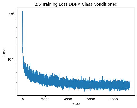
Let's observe the results of the Class-conditioned Unet after 5 and 20 training epochs.
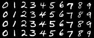
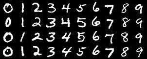
As we can see, the class conditioned Unet generates consistently high quality output that matches the desired class. For reference, the Unet was prompted to generate the digits 0-9 left to right in each row. The Unet acheives this goal very nicely.
This project has been exciting and a great learning experience. Diffusion models are fascinating, and this project has allowed me to get a better idea of their inner workings. I still find it crazy that denoising noise can lead to realistic interesting output images. The articles linked in the project prompt have been interesting reads. For example, I am learning about Runge-Kutta methods in another class, so it was very interesting to learn about the connections of diffusion models to Stochastic Differential Equations solved with Runge-Kutta methods.
I consulted some external resoures when creating this website for instructions on how to write HTML and CSS code. Some of my webpage code is adapted from https://www.w3schools.com/howto/howto_css_images_side_by_side.asp and https://stackoverflow.com/questions/12912048/how-to-maintain-aspect-ratio-using-html-img-tag.