
In this project, I will build a Neural Radiance Field (NeRF) from scratch using PyTorch. A NeRF is a Machine Learning model that learns a scene--typically of some object--using a variety of photos taken from various perspectives. Learning from these photos, NeRF allows us to simulate viewing the object from any perspective. For background information, consider reading the original NeRF paper.
In part 1, we will start with a simpler objective: learn a single photograph. While this alone is a rather silly task (we already know the photo after all), it is a useful warm up for the later implmentation of a full NeRF.
In this part, the model will learn to map pixel locations {u, v} to RGB values in the photo {r, g, b}. We will train the model for a particular photo.


To accomplish part a, we will use a simple MLP model, as shown above, with sinusoidal positional encoding. As found in the original paper, NeRF without sinusoidal positonal encoding will struggle to learn high frequency image components due to neural networks' preference to learn low frequency functions. Sinusoidal positional encoding assists the network to learn high frequency components of the image, since it encodes different frequencies in the pixel locations--information the network will use to learn higher frequency image changes. A higher L value will let the network learn higher frequencies and thus create sharper images. It is recommended to use L = 10; I will try using L = 5 and L = 10. I apply sinPE to the x and y coordinates separately.
We will use the pixel locations and rgb values normalized to the interval [0, 1] for training and inference. After we use sinPE on the input coordinates, we will run the information through a fairly basic Multiple Layer Perceptron neural network with 4 linear layers and layer sizes shown above. Note that the final stage uses a sigmoid activation function in order to output rgb values in [0, 1] as desired.
We will train the model on batches of 10000 randomly selected pixels for 1000 to 3000 iterations. I found that the model is close to fully converged after 1000 iterations, with little change occuring between 1000 and 3000 iterations. We will optimize the model using MSE loss and Adam optimization alogorithm. I tried learning rates of 0.01 and 0.001.
In addition to training loss, another relevant metric of model performance is Peak Signal to Noise ratio (PSNR). With images normalized to [0, 1], there exists the relationship PSNR = 10 * log10(1/MSE).
We will begin by training the model on an image of a fox with hyperparameters L = 10 and learning rate = 0.01.
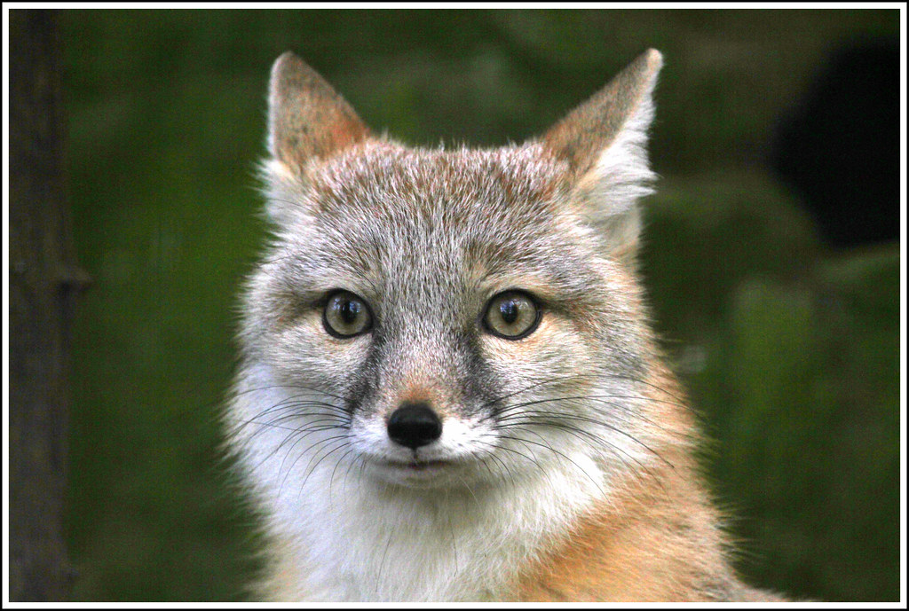
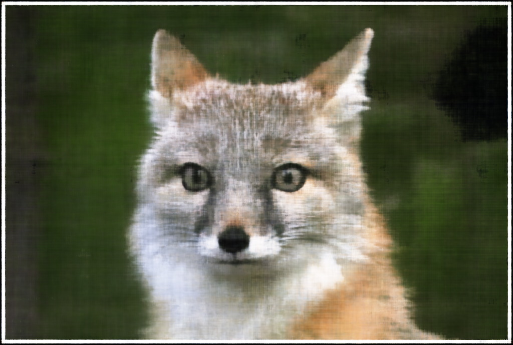

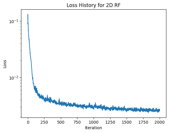
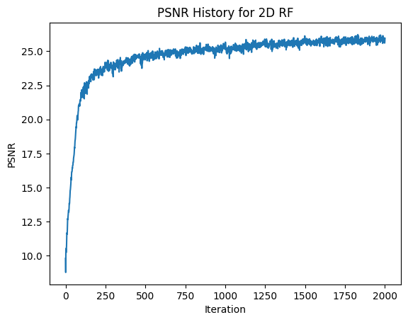
As we can see, the model does a nice job of learning the fox image. It does contain the imperfections of grid-like aliasing in the background and a lack of detail on the fox's whiskers (which are very high frequency).
Next, let's see what happens with hyperparameters L = 5 and lr = 0.01. (Decreasing L compared to the images above).

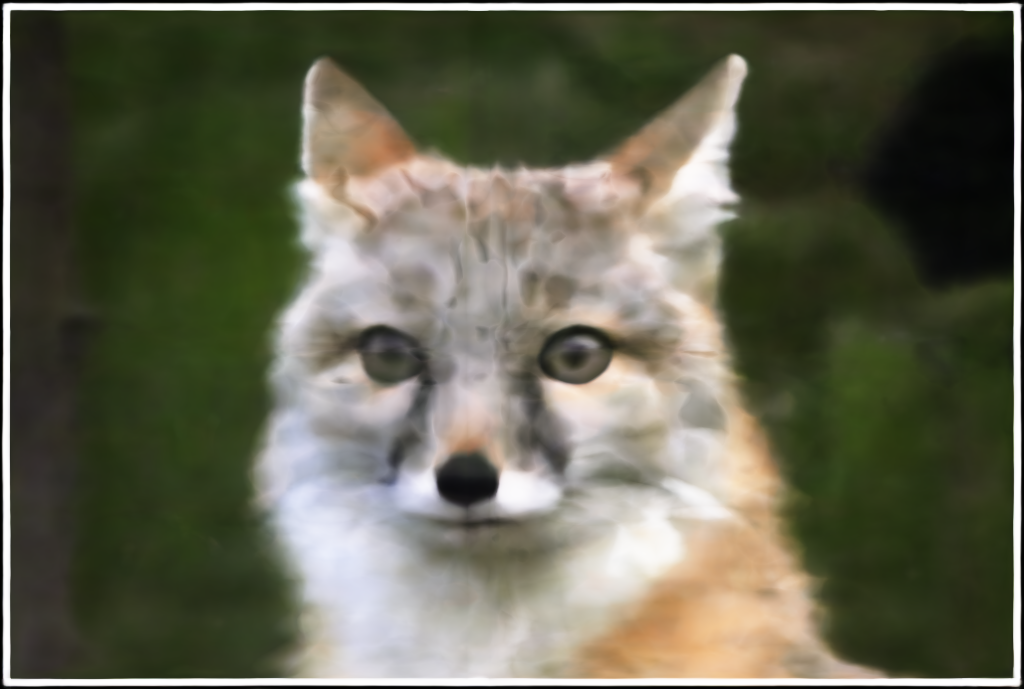

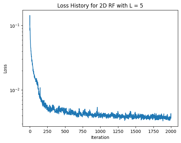
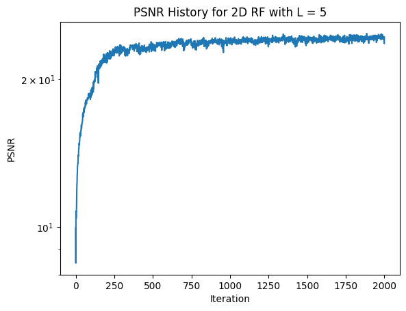
The images learned with L = 5 are clearly worse than with L = 10. When compared to the images learned with L = 10, the images learned with L = 5 have blurry backgrounds, blurry fur patches, and are missing the fox's whiskers. As all of these issues follow from a lack of high frequency image components, it makes sense that these issues were created by a lower L value.
For the next hyperparameter combination to try, we know that L = 10 is a better value than L = 5. In previous training, I have also noticed that the model converges very quickly. Thus, it could perhaps be better to use a lower learning rate. Thus, lets try training the model with L = 10 and learning rate = 0.001 (instead of 0.01).


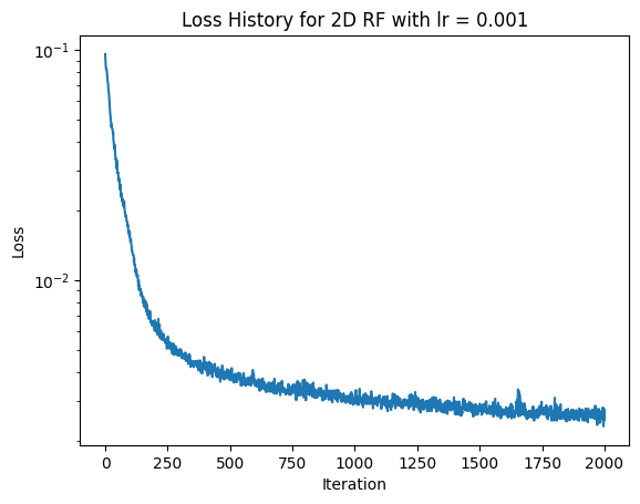
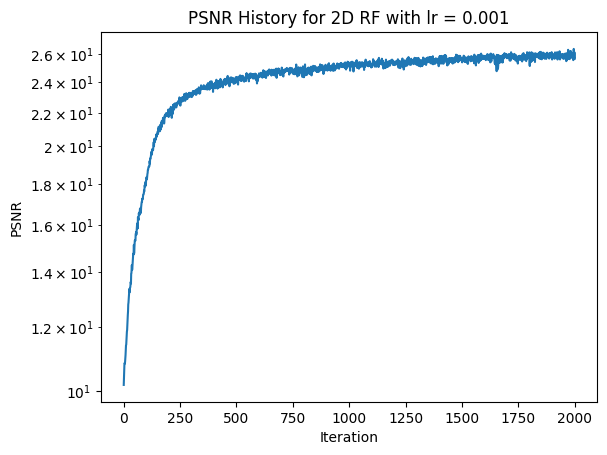
Here we can see that the results are highly similar to when L = 10 and lr = 0.01, except that learning takes more iterations (as would be expected). Thus, I think that the original hyperparameters of L = 10 and lr = 0.01 are the best choice.
Below are all of the images generated under different hyperparameters to compare side by side.


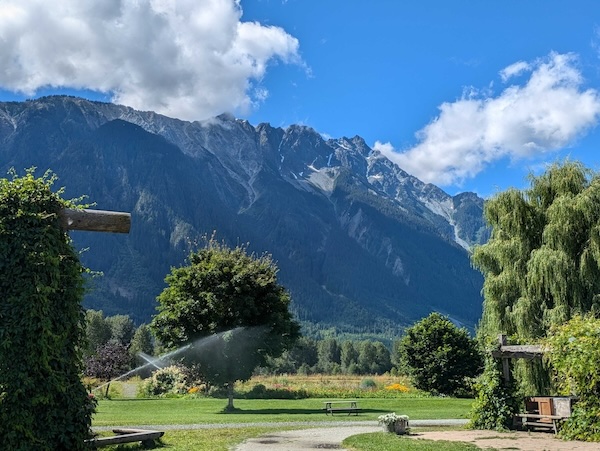
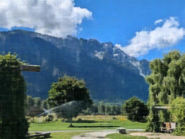
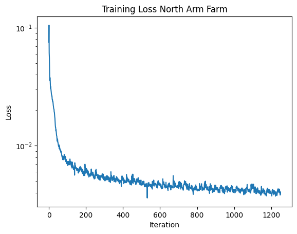
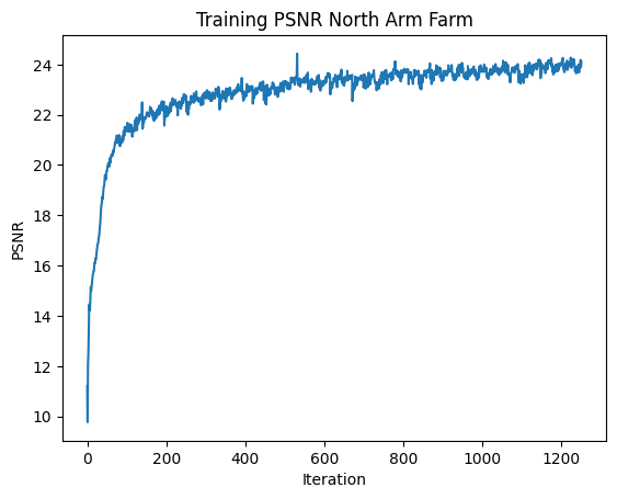
Now I will train the network on a different image, the great North Arm Farm image from Pemberton, BC that recurs throughout my projects. I will use the hyperparameters L = 10 and lr = 0.01. The results are below.

While the previous part yielded a neat result, the next section will be truly epic and has the potential for useful applications. In this section, we will fit a full NeRF model based on the Lego scene in the original NeRF paper. This task will be significantly more complicated than the last, but will allow us to view the Lego from any perspective and ultimately create a 3d rendering of the Lego scene.
By using a dataset with calibrated cameras and known camera locations, we can train the NeRF based on the view of the Lego from various known perspectives. In this dataset, we have 100 training images, 10 validation images, and 60 test images. All images are from unique cameras in unique locations.
In this section, we develop the mathematical infrastructure necessary to generate rays from pixel and camera locations. Rays are integral to the operation of NeRF.
We begin by implementing a straight-forward batched matrix-vector multiplication function to transform coordinate spaces using various matrices. For example, we often use a camera to world (c2w) matrix, which gives the correspondance between points from the camera coordinate system to the world coordinate system. The tranform function will append the bias term to the input coordinates, apply the batch transformation for specified mappings such as c2w matrices, and return the new 3-dimensional coordinates.
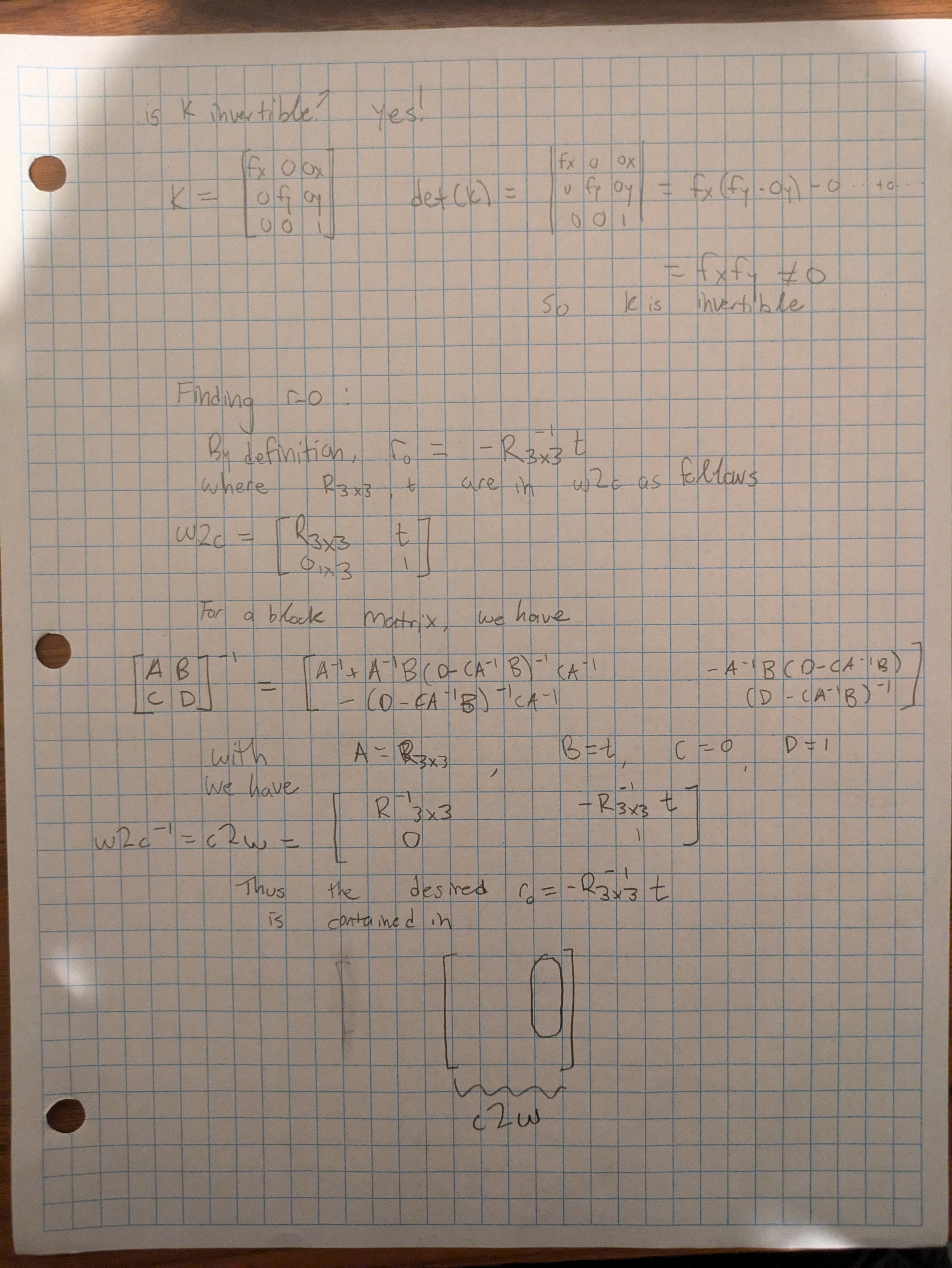
It is important to know the calibration of the cameras. With that knowledge, we can determine the K matrix using the focal length and image size that, along with a distance parameter s, maps pixel coordinates to camera coordinates. pixel_to_camera applies this batched transformation using specified K and s values. This requires solving a system K @ camera_coords = s * pixels_augmented. Since K is only 3x3, I chose to invert K and use batched matrix-vector multiplication. K will always be invertible since det(K) = f_x * f_y > 0, since f_x, f_y > 0 due to the nature of cameras. These calculations are performed in pixel_to_camera().
To complete our goal of determining image rays from pixel coordinates, we need a function to combine these previous functions and calculate the resulting rays. Each perspective of an object can be described by an origin ray and a direction ray. The origin ray specifies the location of the camera in 3d world space, and the direction ray describes the direction the pixel is looking in. Based on the pixel locations, K matrix, and c2w matrix, pixel_to_ray() will calculate the origin ray and normalized direction ray that describe the perspective of the pixel's view. The ray_o vector is defined by entries in the w2c matrix. With some block matrix algebra, we can see that this value is actually given as a vector entry in the c2w matrix. Since the c2w matrix is an argument to the function, we can use a r_o = a 3x1 chunk to c2w to avoid unnecessary calculations. Math shown below.
These batched operations can be implemented using torch.matmul and various squeeze/unsqueeze manuevers.
In this section, we define utility functions and a dataloader that are useful for NeRFs. The dataloader will take in a collection of images, c2w matrices, and K matrix. It is able to randomly sample N rays (with corresponding pixels) for use at each training iteration. We will typically use N = 10000 when training. I implement this by calculating all uv values and rays in all training images upon initializing the dataset. During sampling, I select N rays and pixels at random.
Since we want to incorporate depth information into the model, we will sample along the rays along various depths to get information for the NeRF to operate. We use implement this functionality in the sample_along_rays function. It will return world coordinates at various equally spaced intervals along each ray. During training, we will add a small amount of noise to each interval length to prevent over-fitting. This is implmented using torch.linspace and broadcasting.
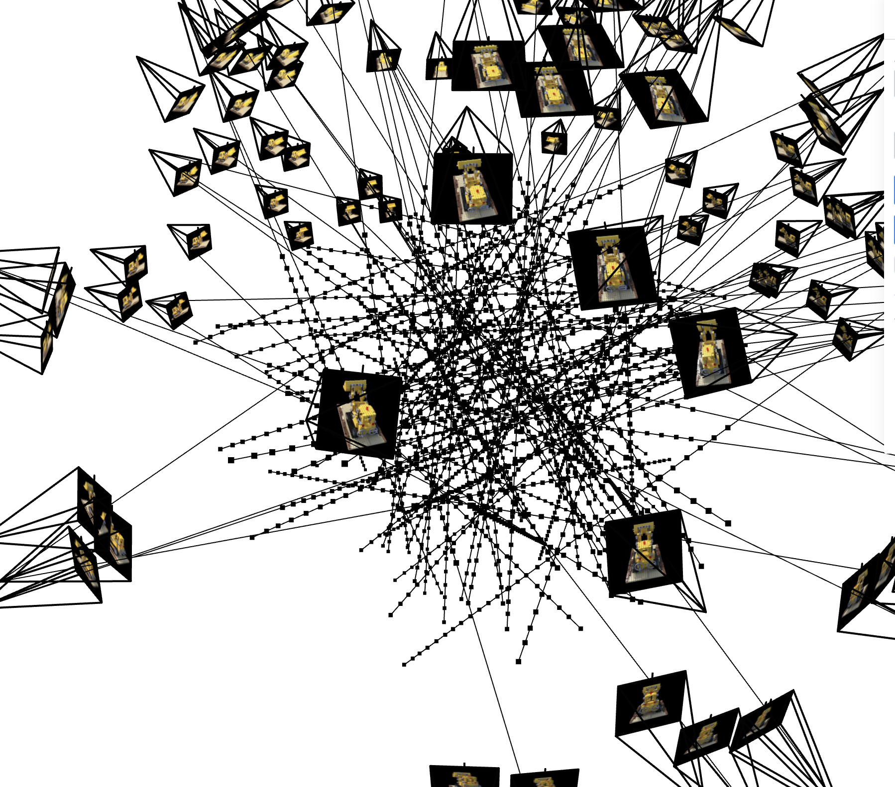
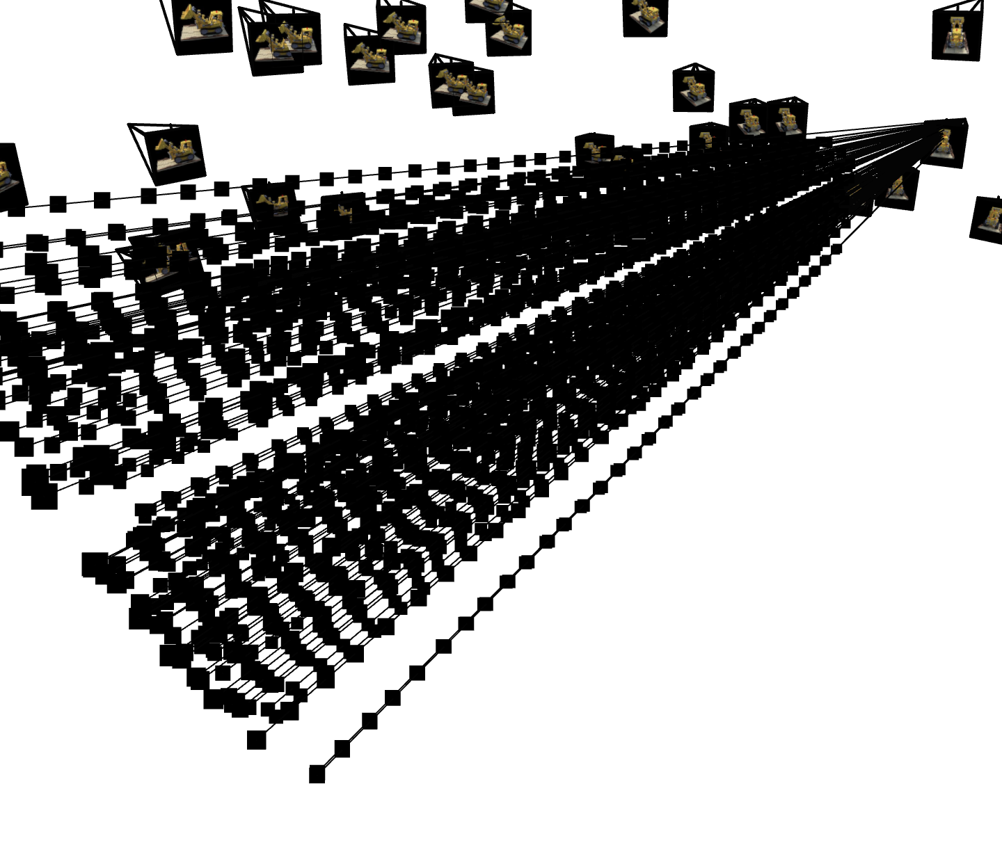
With all of these functions, I will do some visualizations to check for bugs using the nifty Viser package and Viser Studio. The below visualizations gives a scene of the scene we are recreating. The screnshot shows the 3d positions of each camera (including their image), the origin point for each camera, 100 sampled rays, and each sample along the rays (denoted with black squares). Below it we have another visualization that is very useful for debuggging. It shows a dense cluster of rays exiting from the upper left corner of one camera (when viewed from inside the dome of cameras). This ensures that the image dimensions are correct.
In this section, we will build the MLP that underlies the NeRF process. Since this task is much more complicated than the task in part 1, we use a much deeper and more complex MLP. For full architectural details, see the image below. This MLP will take in world coordinates (batched over each ray and samples along the ray) corresponding to the viewing location and batched direction rays corresponding to the direction we are looking in. With this information, the MLP will output rgb values for what can be seen and a density value that describes the transparency for each sample.
This MLP also uses Sinusodial Positional Encoding on both the world coordinates and the directional rays. I use L = 10 for the world coordinates and L = 4 for the directional rays. After the encoding, the MLP uses a large number of linear layers with ReLU activation. As can be seen, the original encodings are concatened to the learned representations at various places throughout the learning process, which helps the model from "forgetting" the input. As before, we use a sigmoid activation function on the last rgb output layer to map rgb values into [0, 1]. On the density output, the ReLU activation forces the output to be positive.

Before we can use our NeRF, we must consider the training target. Our target is to get pixel values at the specified locations. Since our MLP outputs rgba values at various sampling depths, we need a volume renderer to create pixel values at each queried location. The ideal volume renderer works according to the integral below. However, we implement this using the quadrature approximation (also shown below) using the sampled points we generated earlier. Here, sigma is the predicted transparency values and c is the predicted rgb values. I implement the volume rendering in the volrend function, which takes in the output of the MLP and chosen step-size as arguments and outputs the rendered rgb values at each location. This is done using standard operations such as * , torch.sum, torch.cumsum, torch.roll, broadcasting, and unsqueezing.
Since the output of volrend is used in our training loss function, we must be able to backpropagate thru the renderer. Luckily, the volume rendering equation is differentiable and PyTorch makes gradient tracking easy.


Now we are ready to train the NeRF. I'll explain the training pipeline since I was confused myself at the beginning of the project.
During training, we have the pipeline:
Sample rays and pixels -> sample_along_rays -> MLP -> Volume Rendering -> Take Loss with true pixel values
During inference, we have:
Choose desired pixel locations and c2w -> Get rays with pixel_to_ray -> sample_along_rays -> MLP -> Volume Rendering -> Rearrange into image
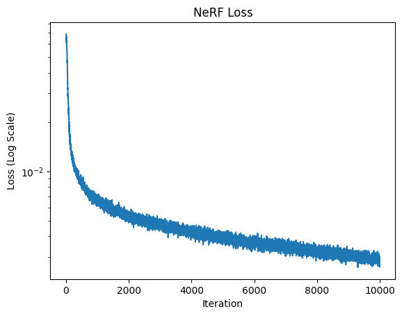
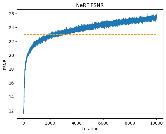
I trained the NeRF using 10,000 iterations with a batch size of 10,000 rays and an Adam optimizer with learning rate 0.0005.
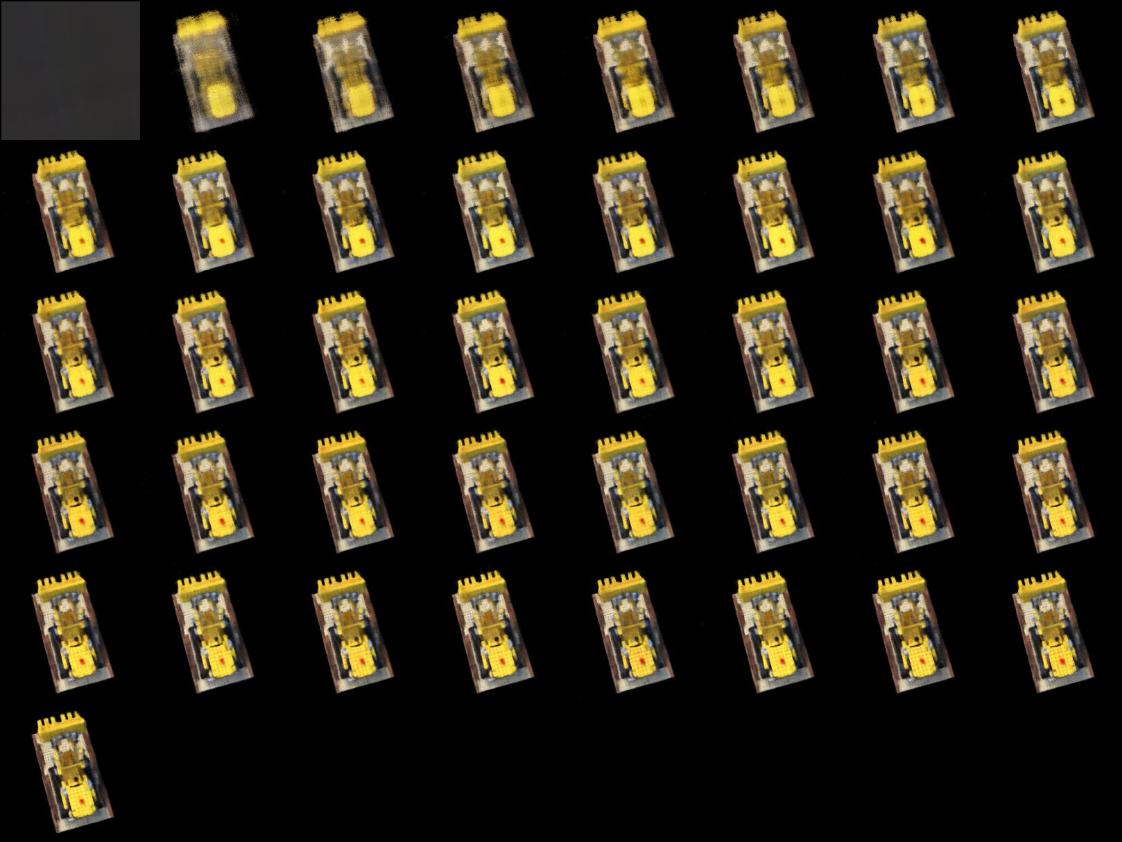
The model acheived good performance on training and testing datasets. After around the 3000th iteration, the model consistently achieved a PNSR above 23 dB. My model acheived a maximum psnr of over 25.86 dB. Below, the loss and PSNR plots are shown, as well as the output over time for validation image 0. We can see that the output image continues to become more detailed and accurate as time increases.

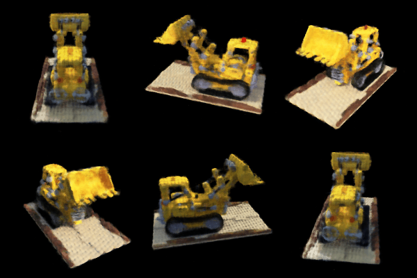
This output is arguably the coolest part of this project. In this section, we used the trained NeRF to generate a GIF based on the cameras in the testing set. The test set cameras form a ring around the lego at an elevation somewhat above the object. We use the model's inference on each camera location to generate a sequence of images moving 360 degrees around the object. This sequence of images forms the GIF. The GIF was generated after training the model over 10000 iterations.
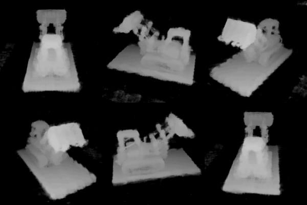
The NeRF model we have already trained contains more capabilities than just those witnessed above. In the inference process, the model generates a density prediction for each sample along each ray. From these densities, we can recover an estimate of the depth along the scene.
To do so, we will use only the density prediction from the MLP along with a modified volume rendering function. I implemented this in the functions depth_mapper and volrend_depth. depth_mapper() performs inference, and only differs from NeRF.sample() by calling volrend_depth rather than volrend. In volrend_depth, we do not use the rgb predicitons from the MLP. In the place of the rgb predictions, we use torch.linspace(1, 0, self.n_samples). This works since T_i * (1 - exp(sigma_i * delta_i) gives the probability that the ray terminates at sample i. Thus, the term forms a probability distribution over all i. Since we want the mapped depth to be bright (i.e. have high pixel values) in areas where the depth is low (i.e. where the ray terminates at a low i value) and darker as the ray terminates at further values (i.e. where the terminating i is large), we see that the weighting term (the linspace) here should be negatively correlated with i. Thus, the decreasing linear weighting given above fits the bill. It would be interesting to try a different depth map--perhaps one based on some characteristic of the derivation of the volume rendering distribution. If I had more time, I would like to try other rendering distributions. However, torch.linspace(1, 0, self.n_samples) provided satisfactory results.
Based on the same testing dataset used to make the GIF above, I use a similar method to create the GIF below showing a depth map of the scene. It also uses the NeRF model trained over 10000 iterations.
This was the most challenging and engaging project I have worked on yet. Given the effort it took to create the model, it was very satisfying to view its successes. Watching training loss decrease is somewhat addictive.
I consulted some external resoures when creating this website for instructions on how to write HTML and CSS code. Some of my webpage code is adapted from https://www.w3schools.com/howto/howto_css_images_side_by_side.asp and https://stackoverflow.com/questions/12912048/how-to-maintain-aspect-ratio-using-html-img-tag.