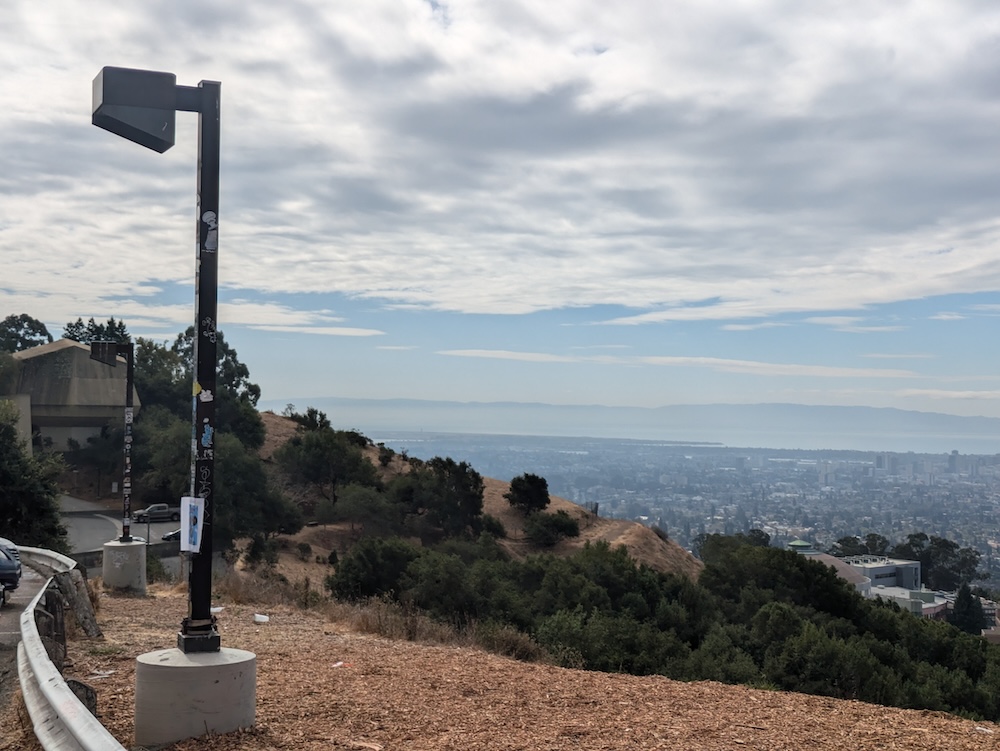
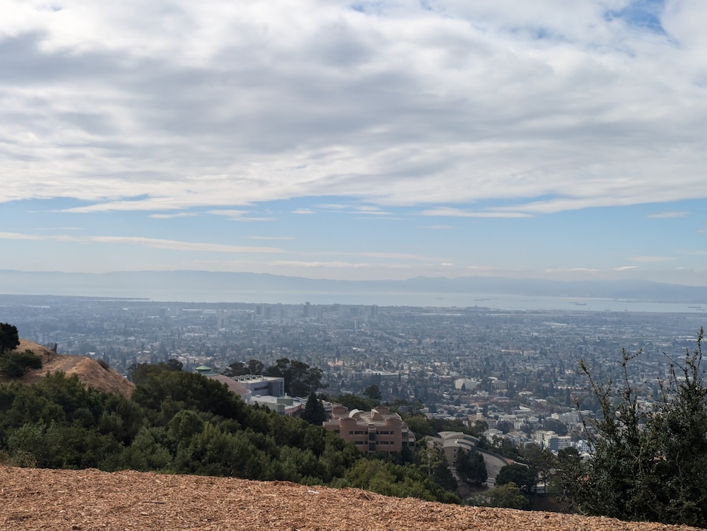
This project, like previous projects, explores image warping. However, this time we are doing so for the purpose of creating image mosiacs. The key to accomplishing this to take photos from the same Center of Projection (i.e. the camera lens is located in the same place) with varying angles of imagery. Thus, these photos will be related by a perspective transformation, also known as a homography. This implies that we can warp the images into a mutual shape such that the images align and the resulting image has a wider field of view. Accomplishing said transformation and warping the images together into a mosiac is the goal of this project.
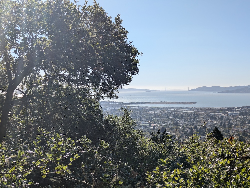
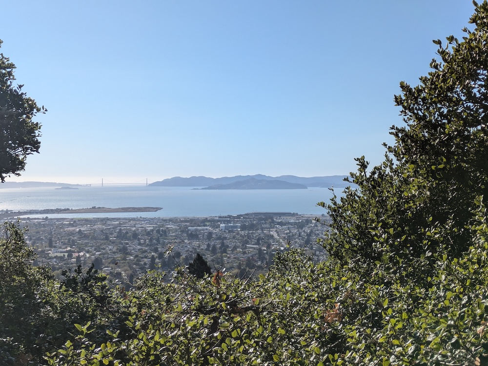
The most important trait of images used in this process is that they have the same center of projection. I am personally using various sets of images of nature scenes captued around the Berkeley hills. Below are the images I will be using.


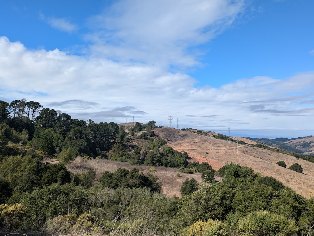
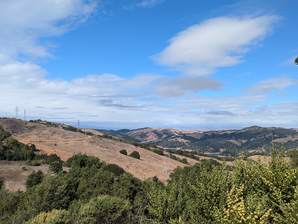
When we will later warp images into mosaics, we need a homography to align the images. A homography is a perspective transformation that tells us how to map the domain of one image such that the image will now align with another image taken from the same center of projection. Mathematically, a homography can be represented as a 3x3 matrix the maps coordinates [x, y, 1] in one image to [wx', wy', w] in another image, where x', y' are the coordinates in the warped image. To accomplish this, we can define coorespondances between the images that we will use to solve for the homography matrix. To do so, I used this tool provided by course staff: Click Here to Find the Tool.
Once we know the corresponding points in the images, we can solve for the homography matrix shown below (my calculations are on paper)!
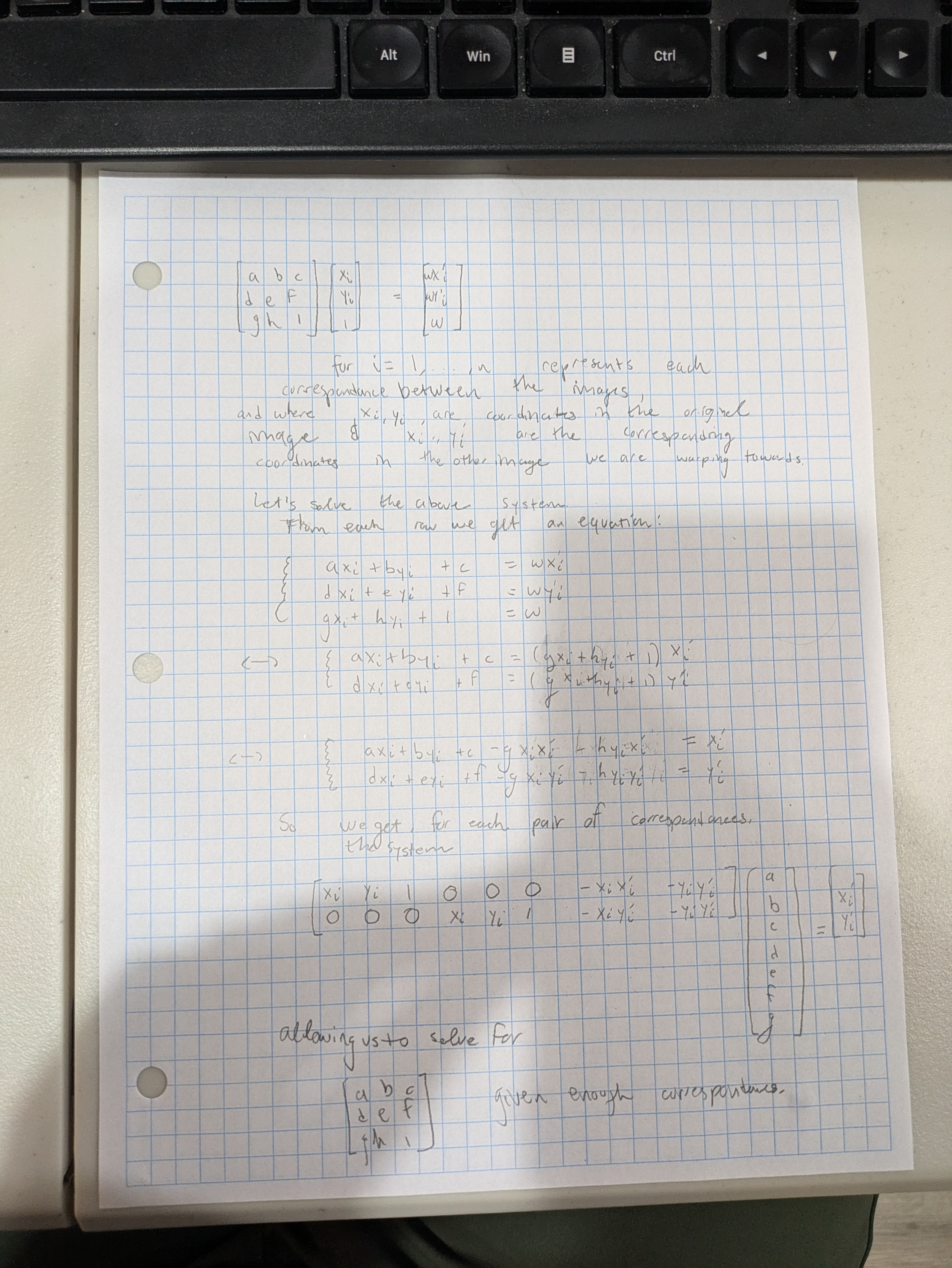
Note that the homography matrix has 8 degrees of freedom. Thus, we need 4 correspondances to solve the system since each correspondance provides 2 equations. However, since points are selected by humans(ie myself), there may be a few pixels of error in each correspondance. Thus, our data is noisy so it is better to use more correspondance points to constrain our solution and make it more robust to noise. Parallels can be made here to Statistical Learning Theory. Thus, I would generally select around 10 correspondance points for each pair of images. Thus, we want to solve the equation Ax = b where A has dimensions (~20, 8) is the matrix of equations I found above on paper, x is the coefficients a, b, ... , h with 8 dimensions, and b is the correspondance points in the other image (around 20 dimenisonal). Thus, the system will be overconstrained. Hence, I use least squares to find the least squares solution for a, ... , h. This can be accomplished using np.linalg.lstsq.
Now, we have our homography matrix.
Equipped with our homography matrix, we can now transform each point in the domain of one image to the corresponding place in the other image--which makes the images align--through the equation H @ [x, y, 1] = [wx', wy', w], where H is the homography matrix and @ is the symbol for matrix multiplication.
Since we ultimately want x', y', we divide by w to find x',y'. It is often the case that some of x', y' will be negative. Thus, I subtract the minimum value over i of xi' from each xi, and I subtract the minimum value over i of yi' from each yi. This ensures that all xi', yi' >= 0. Thus, now all x', y' define positions within an image. Thus, I find the size of the resulting image and interpolate the values at each x', y' to get the original image from the perspective of another image, which will be useful when we make the mosaics.
To warp images, I find all coordinates in the to be warped image, then warp them to their new location using the method in the paragraph above. Then, I interpolate the values at each of the new coordinates using griddata. This is all accomplished with 0 for loops. Since I use 'nearest' interpolation for performance reasons, outside of the convex polygon where the warped images lies are non-sense values filled in by griddata. Thus, I also find the convex polygon that contains the warped image, and I set all pixels outside of the warped image to 0 to eliminate artifacts from griddata. Given on the parameter values passed to warpImage, I will also find the polygon that would contain the overlap of the warped image and the neighbouring unwarped image, which is useful when making image mosaics.
To test our homography capabilties, I will perform image rectification on various images. To do Image Rectification, we start with an image that contains some object that is truly a rectangle but the pixels containing the object in the image are not a rectangle due to the perspective the image is taken from. Then, we warp this image using a homography such that the rectangular object is now also a rectangle in the photo. To do this, I identified the corners of the rectangular image and warp it into a rectangle of a custom size I specify. There is some experimentation with the resulting size of the rectangle to ensure that the aspect ratio is reasonable. Below are some examples of image rectification. In my warp image function, I have a special mode for rectification that allows me to control the output size and domain range of the image. This allows me to isolate just the rectified part of the image. This ability is used below.
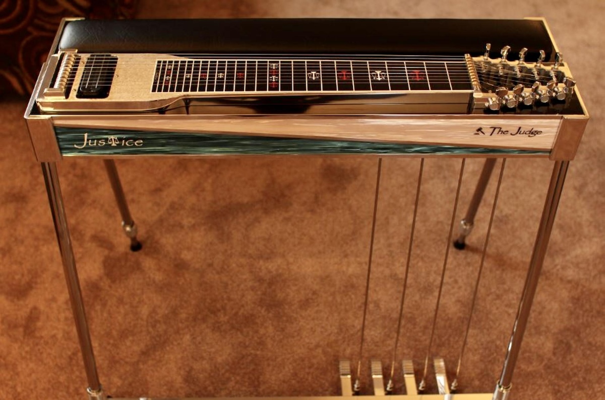


The above image is of an instrument called a Pedal Steel Guitar. Each face on the instrument is truly a rectangle but are not rectangles in the image due to the perspective of the original image. For example, the pixels corresponding to the top of the pedal steel guitar actually form a parallelogram on the 2d image plane while the top of the instrument is actually a rectangle in real life. The lower left photo shows the image rectified such that the top of the pedal steel guitar is now truly a rectangle. This simulates looking down on the image.
The lower right photo is rectified such that the front face of the pedal steel guitar (on its side) has been rectified to an rectangle.
Rectification worked quite nicely in the above images.
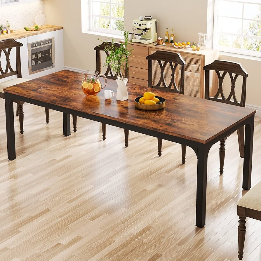
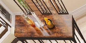
Here, I rectify an image of a rectangular table such that the table is now rectangular. I included some space around the table for reference. Picking out the corners of the table was rather challenging due to its 3d nature.
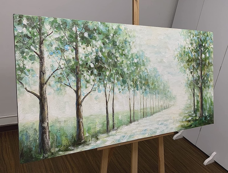
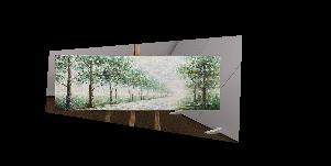
Below, I convert the painting into a rectified image.
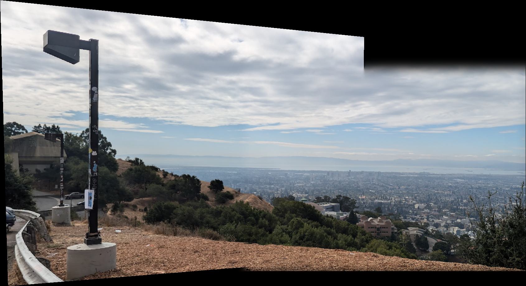
Now for prime time. I am now using the machinery I have built up to manufacture image mosaics. Currently, all of my mosiacs use 2 images. I warp the left image to the perspective of the right image, and leave the right image unchanged. I use where the corners of the left image are mapped to calculate the overall shape of the output image. My image mosaic code calls my image warping code. Likewise, I also adjust the transformed coordinates such that all of the warped image's coordinates are non-negative, thus allowing it to fit into the resulting image.
I align the two images using the minimum corner values of the left image. We know that with the coordinates of the left image unchanged, the points in the image will align with the points in the right image when the right image has no shifting. This is something I confirmed earlier on in the project. Thus, when we shift over the left image coordinates by subtracting the minimums, as detailed in the section above, we can also simply move the right image over by the same amount and the images will still align.
The most difficult part of image mosiacs and of project 4a is to determine how to blend the images together to eliminate edge artifacts. I tried many methods, such as plain overwriting (for a benchmark), alpha channel blending using the distance from the center of the image, and blending with Laplacian stacks with various parameters and masks. I found Laplacian blending to be the most effective. I found two different masks that were effective, often with one of the masks being superiour for certain mosaics. Thus, I would choose the mask with the superior performance on a particular mosaic. Ultimately, here are my two different systems for blending:
1. Set the mask to be 1 in the area inside the unwarped right image such that there is about 10 to 30 pixels (depending on the image) from the edge of the mask's 1 values to the side of the unwarped image. This offset is important to avoid black lines at the intersections of the two images. I then used 3 of Laplacian Stack for the two images to blend and 3 or 4 (hyper parameter) levels of Gaussian Stack for the mask. Generally, this method was more succesful. With 4 levels of Gaussian Stack, I will use the mask in 1 layer further down in the mask Gaussian stack in order to get smoother blending.
2. Set the mask to be 1 in the area inside of the warped left image. I would use the corners of the warped image to find the polygon containing the image. To avoid black lines, I would set the right hand corners of the polygon (where the intersection with the other image is) to be [30, 30] pixels inside the warped image from the actual corner. With this method, I used 3 levels of Laplacian Stack for the two images to blend and 4 levels of Gaussian Stack for the mask. When blending, I will use the mask in 1 layer further down in the mask Gaussian stack in order to get smoother blending.
In both cases, I have found that using small kernels is sufficient for blending and provides quicker runtimes.
I then would use weighted averaging, as in Project 2, to combine the two different portions of the image. Before blending, I make an image the same size as the output image containing just on the particular images for use when blending and finding the Laplacian Stack.
My approach to creating the Laplacian and Gaussian Stacks is the same approach I used in Project 2.
Click here to see my description from Project 2
The left two images are images I will be using to create the mosaic, and the right image will be of the mosaic itself.








In part B, we are extending the ideas we developed in part A to include the ability to automatically determine features and match images, reducing the amount of human labor needed in the process. With the exception of RANSAC, I am implementing image matching as described in the Brown et al. paper on the subject. I also implement RANSAC myself, which I learned in lecture. I'll walk readers through the process of automatically determining image feature matches.
Our journey begins with the Harris Interest Point Detector. The Harris method analyzes how much small areas of images change in certain directions in an attempt to find corners. The concept is that only corner points will produce differences in all directions when moving the sliding window. For examples, points on lines will not produce differences in one direction (the direction moving along the line). While not all the points Harris finds are what a human might consider a corner, many are still relevant points of interest for matching purposes. I am using the Harris code provided by course staff. This code finds the pixel that creates the maximum Harris score such that each point is seperated by at least 1 pixel from another point (i.e. the maximum over each 3x3 window). Below are examples of the points the Harris algorithm finds.

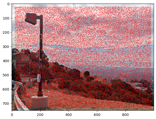
As we can see, the number of Harris points is huge and includes many irrelevant details. In the current form, these points will not be useful to create image mosiacs. This leads us to the next topic
Adaptive Non-Maximal Supression (ANMS) is heuristic algorithm that locates the most important image points. ANMS filters out Harris points based on the distances to other significant points. ANMS works by determining, for each point, the minimum radius from that point to another point that is significantly greater in strength. Significantly greater in strength means that f(x) < c_robust * f(y) , where f(.) maps a harris point to its corner strength, x is the corner is question, y is a distinct corner from x, and c_robust is a hyper parameter to be chosen. As recommended in the paper, I use a value of c_robust = 0.9, which worked well for me. To be precise, the exact formulation of the minimization problem is given below. Note that the absolute value should be replaced by the L2 norm squared. Since norms are non-negative and f(x) = x ^ 2 is monotonically increasing over (0, inf), it is equivalent to replace the norm with the squared norm in the below minimization problem.
One interpretation is that ANMS assigns radii to points based on how locally significant the point is. A larger radii means that the point is significant for a larger area. The aim of ANMS is to filter the number of correspondance points and find the most useful corners. Thus, we take the N points with the greatest radii value found by ANMS, where N is a hyper parameter. For image stitching, I generally found N = 100 to provide plentiful correspondances. However, one image pair required a greater N value, so I used N = 500 with that image pair. Taking the points with the largest radii means that we are keeping the most significant points.

Below are the results of ANMS filtering the Harris points for different values of N


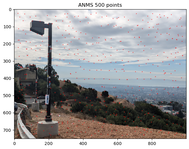
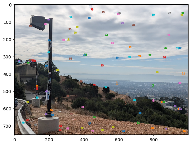
As we can see, ANMS does a very nice job of indentifying important points that are well spaced throughout the image. Occasionally, there are some points that are very close to each other. One may wonder how it is possible to have points close to eachother remain after ANMS. It is because these points have very similar corner intensities, so neither point satifises the optimization constraint for the other point. Thus, the minimally distant point from each point is some other point(s) further away, allowing both points to have sufficient radius to be in the top N ANMS point radii.
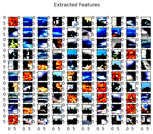
Now, we aim to match features between different images in order to obtain correspondances. Thus, we need some way to summarize each corner that is invariant to various insignificant changes in the images, such as gain, intensity, and scale. To do this, we use the method described in section 4 of the research paper. We will summarize the 40x40 pixel area around each corner as an 8x8 image for efficiency then apply normalization. For each corner we will repeat the following steps:
1. Extract the 40x40 pixel region surrounding the corner such that the corner is in the middle.
2. Apply a Gaussian Blur to prevent aliasing when downsampling. Below, I calculate the proper sigma in greater detail.
3. Take each 5th pixel in a rectangular pattern in order to get a 8x8 feature desciptor. Due to previous blurring, this descriptor is nice and blurred to accomadate for different image scales.
4. Finally, normalize the descriptor such that the descriptor has mean 0 and standard devation 1. Thus accomadates matching between images with different gains or itensities during the image creation process.
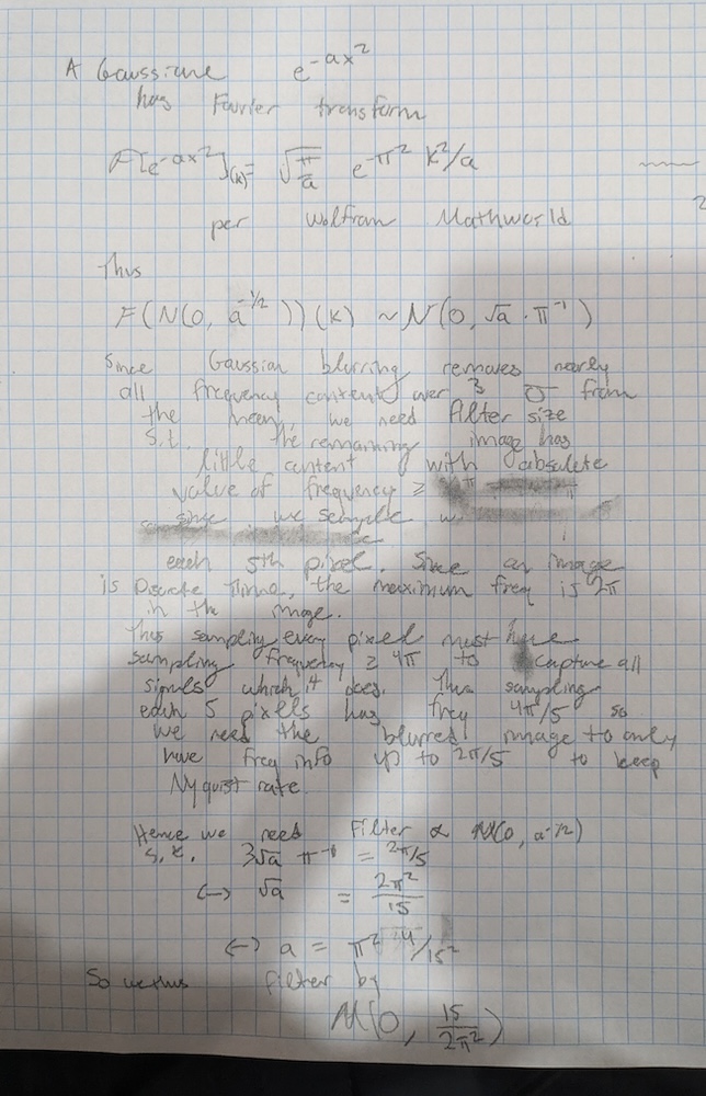
We must decide what sigma to use when blurring the corner surrounding region to get an 8x8 descriptor. Advice on picking this sigma is noticeably absent from the paper. Hence, I returned to my Signals and Systems days and performed a Fourier Analysis to determine what sigma value to use. In the below mathematics, I choose the value of sigma such that virtually all frequency content above the Nyquist frequency for the downsampling will be eliminated. For this calcuation, I use the fact that virtually all of the measure of a Gaussian lies within +- 3 standard devations of the mean. Since convolution in the spatial domain is equivalent to multiplication in the frequency domain, we can choose the sigma parameter of the Gaussian such that +- 3 std in the frequency domain equals the Nyquist frequency of the downsampling. I use the Fourier Analysis formula for a Gaussian as given in Wolfram MathWorld. Ultimately, I find that the sigma value of the Gaussian blur in the spatial domain should be 15/2/(pi ^ 2). This value worked well for me in practice.
Below are the results of finding the feature descriptor for each corner in the ANMS Top 100 corners. Note that many of the values have been clipped at 0, 1 by Matplotlib so the real descriptors will be less uniform in value than how they are presented.
Once we calculate the feature desciptors for each image, we need to determine which descriptors describe corresponding points in the images. My approach for this section is based on the method described in Section 5 of the Brown et al. research paper. This technique leverages nearest neighbour matching. The algorithm works as follows:
1. For the first image, perform the following steps:
1a. For each feature descriptor, find the nearest neighbour and second nearest neighbour feature descriptor in the other image, where distance is defined as the Sum of Squared Differences like in the dist2 starter code provided. If the ratio of the distance to the nearest neighbour and the distance to the second nearest neighbour is below a cutoff (I use the hyper paramter value of 0.25 -- rationale is below), identify the points as a potential match.
2. For the second image, perform similar steps:
2a. Likewise: For each feature descriptor, find the nearest neighbour and second nearest neighbour feature descriptor in the other image, where distance is defined as the Sum of Squared Differences like in the dist2 starter code provided. If the ratio of the distance to the nearest neighbour and the distance to the second nearest neighbour is below a cutoff (I use the hyper paramter value of 0.25 -- rationale is below), identify the points as a potential match.
3. Keep all matches that are identified as matches in both steps 1a and 2a. I found that imposing the mutual match requirement greatly improved feature matching.
As mentioned above, this algorithm also requires choosing a hyper-parameter. This hyper-parameter controls the maximum allowable ratio of nearest neighbour distance to second nearest neighbour distance for a pair of points to be considered a match. Figure 6b in the Brown paper shows a real-world case study on the probability densities of true and false matches. The points we label as matches are likely to be used to determine the homography for image warping (if the points pass RANSAC). Since we fit the homography using least squares--a technique highly susceptible to corruption from outliers--having any incorrect matches can be very dangerous. Even a single incorrect match can cause a poor homography to be found. Additionally, since we typically start with hundreds of potential matches, it is acceptable if we eliminate some correct matches. Thus, I chose a hyper parameter value of 0.25, since 0.25 allows almost no incorrect matches while allowing a healthy amount of correct matches. Using the hyper parameter value of 0.25 has been successful for me.
The intuition for this algorithm (known as Lowe's trick or the Soviet Grandmother Wisdom) is that the 1-NN may be a match while the 2-NN is not a match. If the point is a match, the distance to the 1-NN should be significantly less than the distance to the 2-NN. By the contrapositive statement, we can eliminate incorrect matches.
Below are the results of applying feature matching on our demo images.
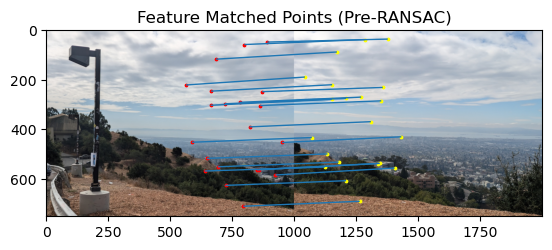
All of the matches appear to be quite good to me.
As mentioned above, having any incorrect matches can be very dangerous to fitting a correct homography. Thus, we will also use RANSAC to elimate any remaining incorrect matches after the previous Feature Matching step. To implement RANSAC, we randomly draw sets of 4 corners (without replacement) from the matches, fit the resulting homography, and take note of how many points are accuractely mapped by the homography within some tolerance (another hyperparameter to tune! I'll call it epsilon). We repeat this process a large number of times. I found 300 iterations sufficient to reliably find high quality homogrpahies; however, it is not uncommon to use more iterations. If we have drawn all points but still need to perform more iterations, I reshuffle the lists of corners and contintue the loop of drawing four corners without replacement. The points that are accurately mapped by the fitted homogrpahy at each step are known as "inliers". We ultimately keep the largest set of inliers as our matches. We will fit the homography to these points.
I tried several different values of the epsilon hyperparameter. I intially began by using small values such as 0.05 and 0.1; however, this tolerance would not find any inliers other than the four points used to fit the homography. I learned that I need to be more tolerant of small errors by RANSAC. I found that a epsilon value of 4 would allow for many matching points to be found while still removing outliers.
Below are the results of applying RANSAC to the point set shown above.

Due to the strength of my previous matching algorithm, we can see that only a few points are eliminated by RANSAC. It appears that all kept points have strong correspondance with each other. Ultimately, 19 points were kept, which is a healthy number for fitting the final homography.
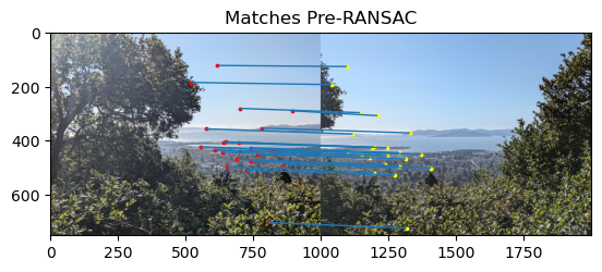
Since my matched points above were already so well matched, the RANSAC algorithm did not get the oppurtunity to prune much. Thus, I generated more RANSAC comparisons below with a pair of images that were somewhat more difficult to align. We can see that the pre-RANSAC image has a few poor matches. For example, there is a match between two points in the sky that is incorrect. We can see that these incorrect matches are filtered out by RANSAC.

With this background material out of the way, now we can produce image mosaics automatically. I combined all of the previous functionality into one function so that we can now create image mosiacs with one function call and only a pair of images and some optional hyperparameters as arguments! How cool is that!
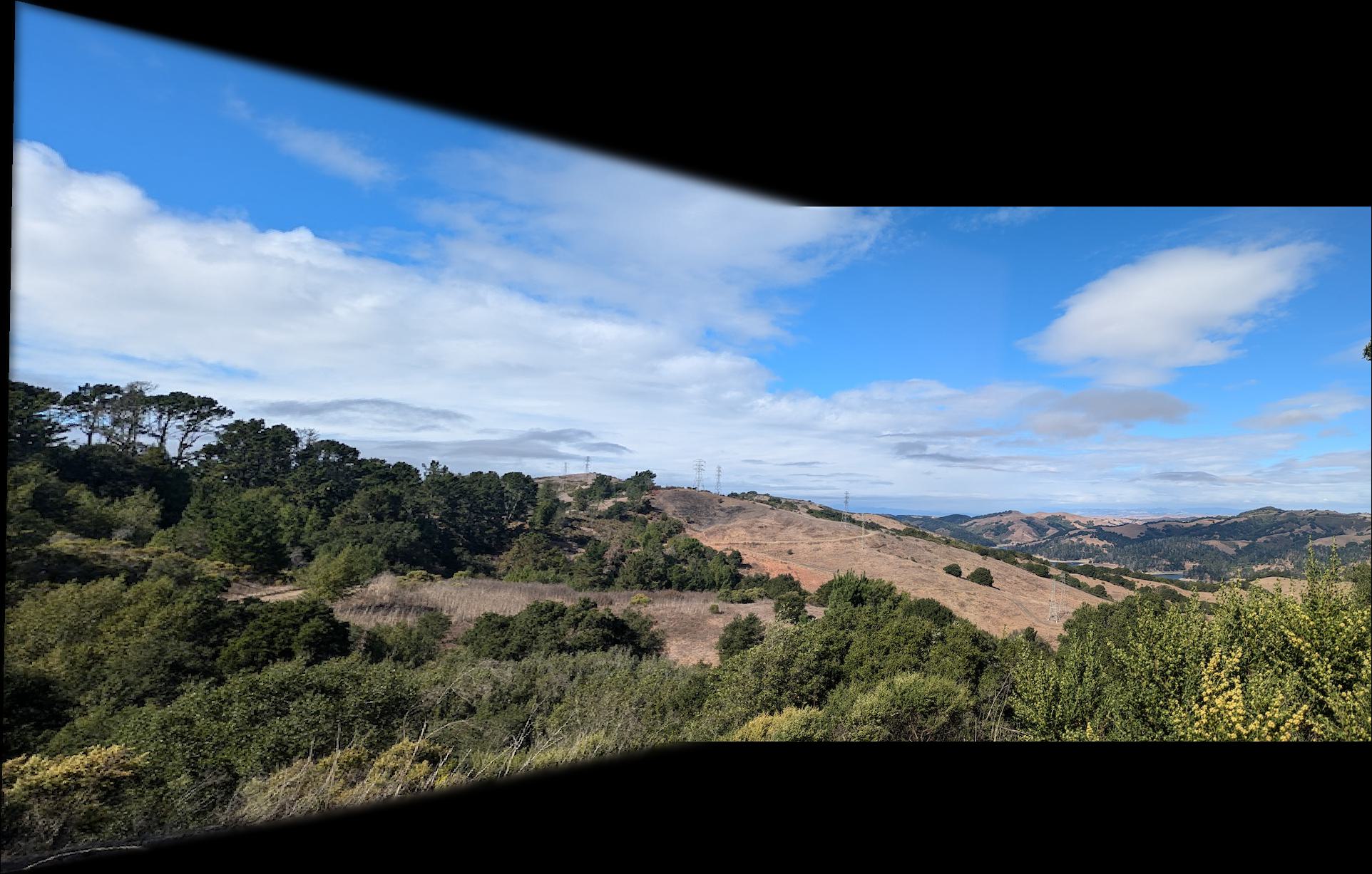
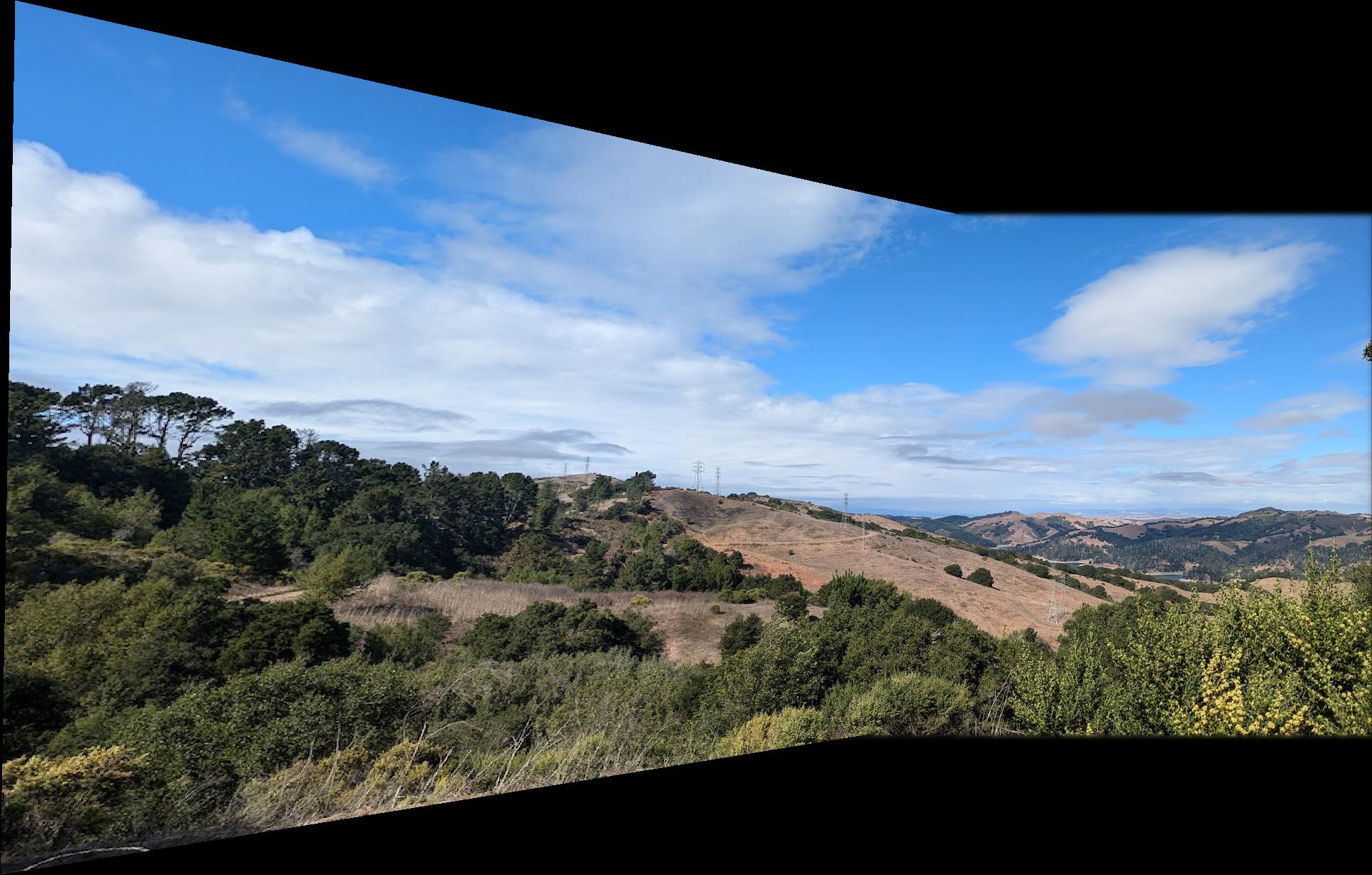
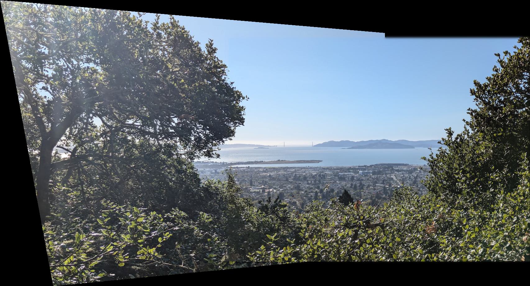
Let's take a look at the results. I'll use the same images I created image mosiacs for manually, so that we can can judge how well the automatic stitching performed.

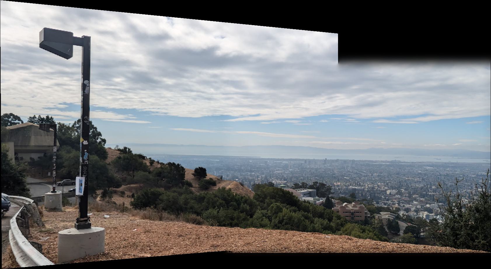

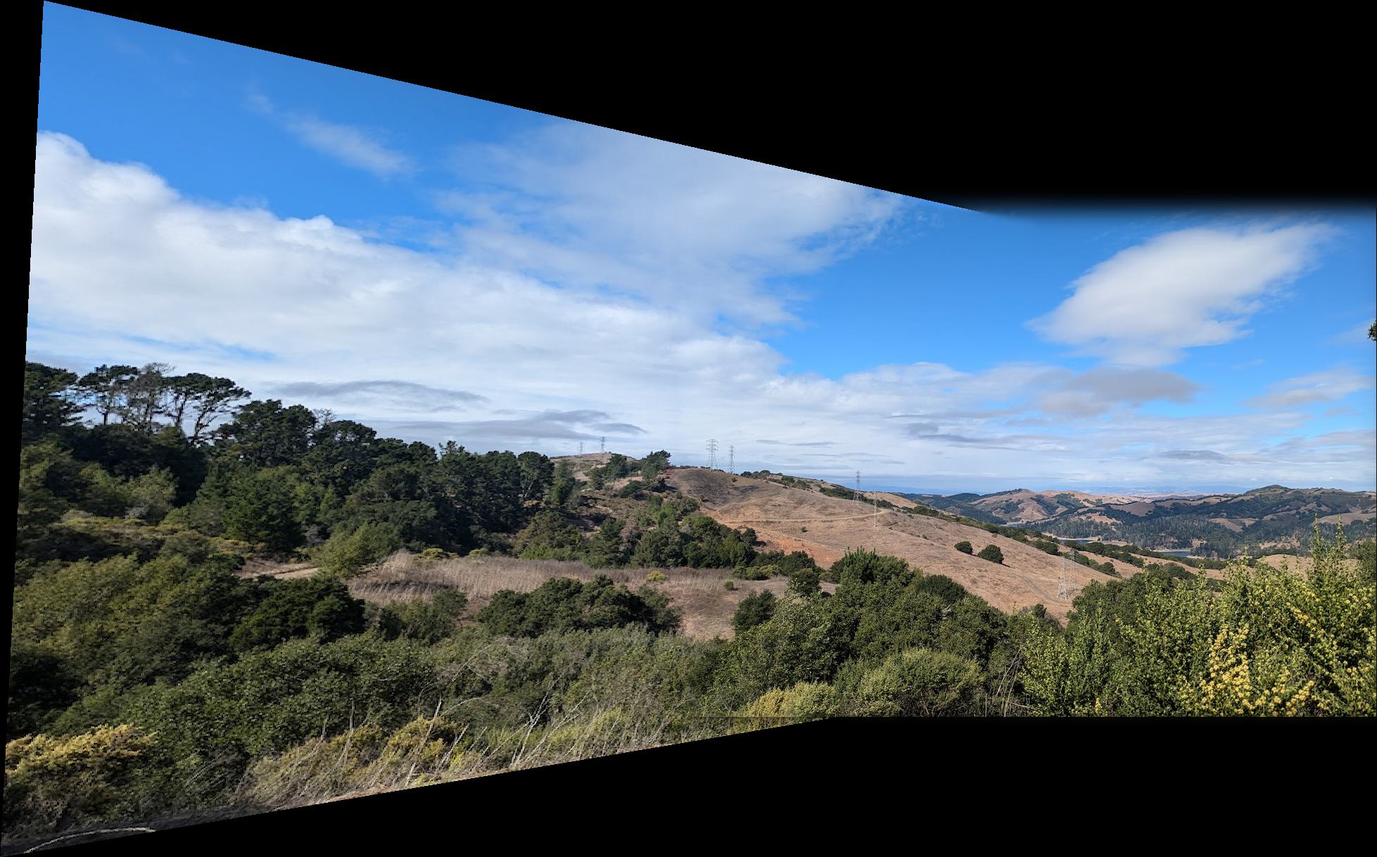

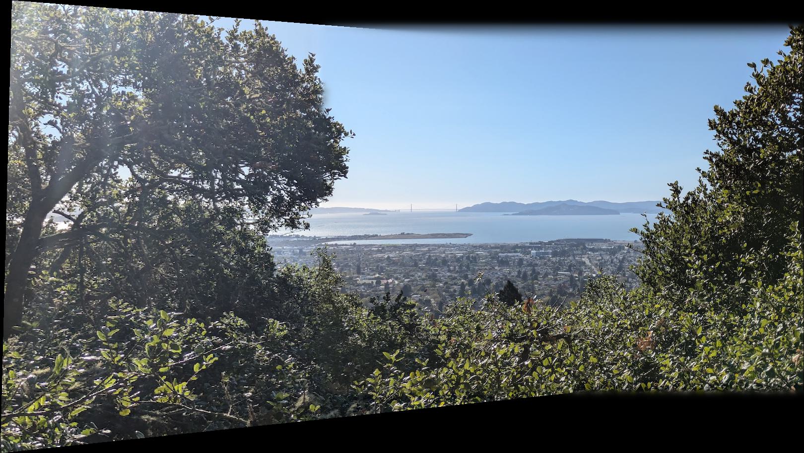
In my opinion, these automatically stitched mosaics look very nice and comparible to the manually made mosaics. In all three cases, I can tell not tell a difference in the alignment of each image pair. However, the difference in the perspective of the left image in the third mosiac between the manual and automatic mosaics is perplexing. In the third mosaic, the viewer can see that the shape the left image is warped into is different between the auto and manual mosiacs. However, the image pair appears to be well aligned in both images. I can not tell where the image seam is in either mosaic, indicating a high quality of alignment between the images.
Note that sometimes the automatic and manual mosaics used different blending techniques which can affect the boundaries of the mosaics.
This entire project has been really cool to complete! I have especially enjoyed Part B and implementing an algorithm with enough intelligence to find matching features that robustly create good image mosaics. If I had to pick one thing, I am the proudest of my implementation of feature matching and the way I encorparated nearest neighbour search manually. I find it very cool how we can abstractly extract information about points of interest and match them based on this information.
I consulted some external resoures when creating this website for instructions on how to write HTML and CSS code. Some of my webpage code is adapted from https://www.w3schools.com/howto/howto_css_images_side_by_side.asp and https://stackoverflow.com/questions/12912048/how-to-maintain-aspect-ratio-using-html-img-tag.
When solving for the equation of the homography matrix, I was influenced by materials provided by course staff--in particular, the site of Alec Li. I derived the equations myself; however, given the recommendation by course staff, I viewed Alec Li's page to see examples of image mosaics when begininning on the project. There, I observed his solution for the homography system of equations, which may have subconicously affected my approach to solving the system myself.
I used the formula for the Fourier Transform of a Gaussian as given on Wolfram MathWorld here.
I would like to emphasize that all of the code for image processing is of my own creation.